Week 1 Lab: Introduction to R and Tableau

Learning Objectives

This lab contributes to Course Objectives 2, 3, & 4
Open R/Rstudio and ensure it is functioning properly
Get oriented with RStudio
Conduct basic calculations in R
Navigate directories from within R
Read in an external data set in R
Load a package in R
Create your google site and a project page
Apply for Teableau academic license
Download Tableau desktop and ensure working correctly
Register for Tableau public

Introduction to R

Welcome to the world of R programming! R is a powerful and widely used programming language in the field of data analysis and statistical computing. It is known for its vast collection of libraries and packages that allow users to easily perform complex data manipulation and analysis tasks.

Before we get started, you will need to install R on your computer. You can download the latest version of R for free from the official website https://cran.r-project.org/. Once the installation is complete, you will also need to install RStudio, a popular integrated development environment (IDE) for R. You can download RStudio from the official website https://rstudio.com/. Alternatively, you will have access to a version of RStudio on a CSU server that you can access via web browser here: http://darecompute-01.aggie.colostate.edu:8787/. I will provide you with log in credentials in class.

RStudio provides a user-friendly interface for working with R and offers a variety of features to make working with R easier and more efficient. Open up RStudio and you should see something that looks like this:

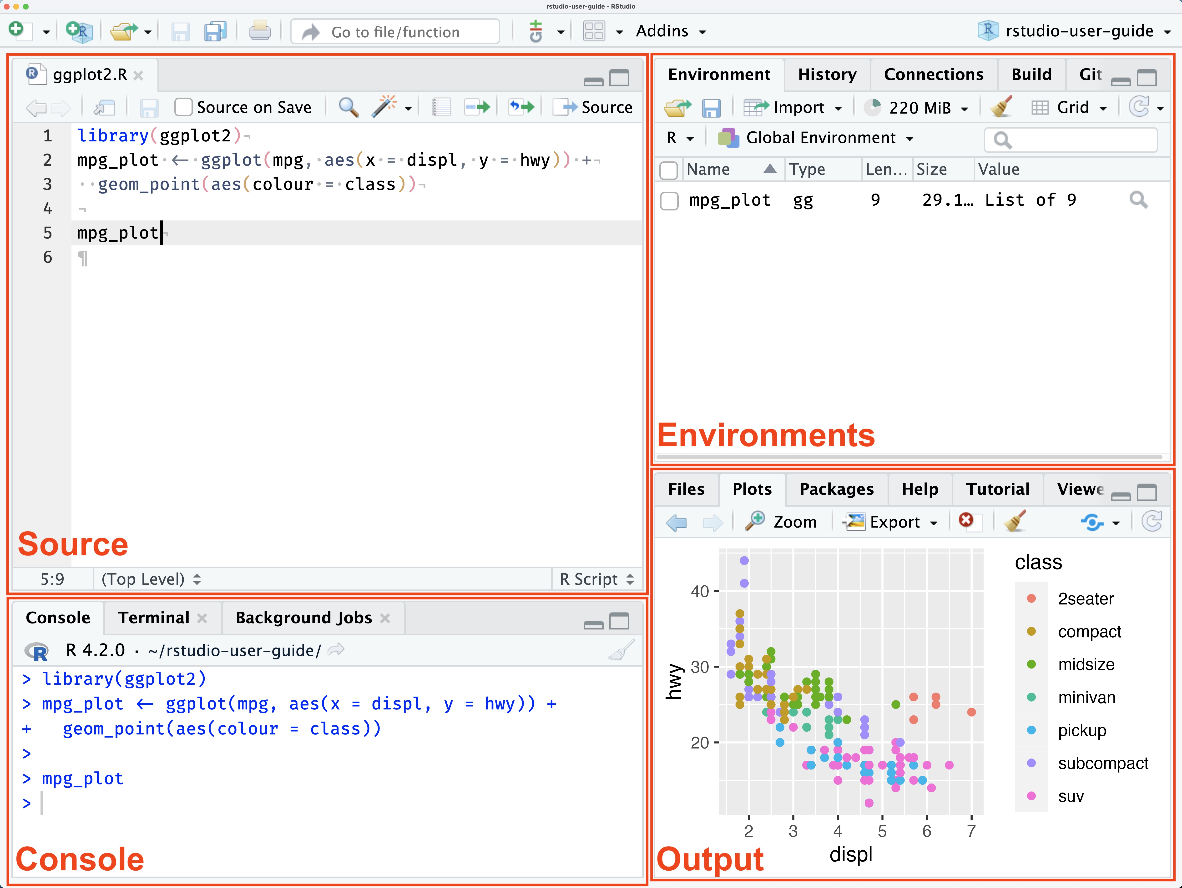
The RStudio interface is divided into several panels:

The Console panel is where you can enter and run R commands.
The Source panel is where you can open and edit R scripts, which are files that contain R code.
The Environment and History panels display information about the current environment and command history.
The Files, Plots, Packages, and Help panels provide access to various resources and tools.

Now that you have both R and RStudio installed and running, let’s dive into some basic concepts of the R programming language.

First, R is an interpreted language, which means that you can enter commands directly into the console and see the results immediately. You can start the R console by opening RStudio and clicking on the “Console” tab.

Basics

To assign a value to a variable in R, you can use the assignment operator <- or = like this:

x <- 5

x = 5 #Does the same thing

Here, we have created a variable called x and assigned it the value of 5. Anything following the hashtag on the same line is interpreted as a comment and not executed. Once you assign a variable a value, you can see it in your environment panel. You can use the print() function to display the value of a variable:

print(x)

[1] 5

Stop and open a new R script. Because R is a command-line application, we can write a script (i.e., text file) with a sequence of commands. There are many benefits to scripting. First, you can save a record of the commands if you need to reproduce the analysis. Second, you can share it with others so they can reproduce it. Third, you can easily change a part of your script to see what happens.

You can also perform basic arithmetic operations in R using the standard operators (+, -, *, /):

y <- 3
z <- x + y
print(z)

[1] 8

First, we assign the variable y the value 3. Then, we assign z the value of x (assigned 5 earlier) plus y (just assigned 3), which sum to 8.

Comprehension check: Try assigning the variables a and b different values and dividing them.

R also has a wide range of data types, including: numerical, character, and logical. Variables can be different datatypes. Collections of variables are called a vector - a one-dimensional array of data. You can create a vector using the “c()” function, which stands for concatenate. A vector may only contain one type of data.

numbers <- c(1, 2, 3, 4, 5)
characters <- c("a", "b", "c")
logical <- c(TRUE, FALSE, TRUE)

Indexing

A single entry in a vector is called an element. You can access elements of a vector using the square bracket notation:

print(numbers[1])

[1] 1

Comprehension check: Try accessing a different element of the vector numbers or one of the other vectors.

You can also access series of elements in the vector. To access a continuous range of values use the colon :

print(characters[2:3])

[1] "b" "c"

You can even use a vector of index values to call discontinuous subsets of the vector.

print(characters[c(1,3)])

[1] "a" "c"

Depending on the datatype, there are functions that operate on the vector. For example, you can sum the elements of the numeric vector numbers.

print(sum(numbers))

[1] 15

Comprehension check: Can you sum the numbers of the vector characters? How about logical?

Challenge: Can you figure out how to calculate the product of the vector numbers?

You can also add, subtract, multiply, and divide all of the numbers in a vector

print(numbers+5)

[1]  6  7  8  9 10

Or add, subtract, multiply, and divide numbers of equal-length vectors

print(numbers + numbers*2)

[1]  3  6  9 12 15

data.frames

Using R like a fancy calculator is intended to help you understand how R works. R is generally used to analyze data sets. Data sets are collections of equal-length vectors in a table or what R calls a data.frame. Here is a simple example:

print(data.frame(a=c(1:3),
                 b=c(4:6),
                 d=c(7:9)))

Where a,b,d are the column or variable names and the 1,2,3 on the far left are row numbers.

You can build a data.frame using the vectors above and assign the object a name.

df <- data.frame(numbers=numbers[1:3],
                 characters,
                 logical)

print(df)

  numbers characters logical
1       1          a    TRUE
2       2          b   FALSE
3       3          c    TRUE

Comprehension check: Why did I subset the vector numbers?

Reading data

Creating data.frames by hand is tedious. Fortunately, R has some utilities to read data stored in certain files types. Before we explore R’s ability to read data, we must understand how R interacts with the computer’s file system. At any point in time, you are in an active directory (similar to windows explorer or macos finder). You can ask R to tell you the current working directory (where R is looking at the moment).

getwd()

[1] "/Users/judebayham/Documents/git_projects/csu-arec-330.github.io/materials/unit_00/week_01"

The response to this command will depend on the directory structure on your machine. You can navigate your directory structure using the command setwd(). When you have multiple projects with multiple files on your machine, it will be important that you understand R’s working directory and how to change it. The syntax will depend on whether you are on a windows or mac. First, locate the data file that you downloaded for this exercise. You will treat this like the project directory and instruct R to navigate your directory structure by typing the path to the directory in the setwd("directory/subdirectory1") command. The path needs to be in quotes to tell R that you are inputing characters and not variables.

This video describes a computer’s file system and organization: https://www.youtube.com/watch?v=hUW5MEKDtMM

To read data into R, we will use another function built into R. We will be reading a file type called comma-separated values denoted by the file extension .csv. The commas separate the variables, so R knows where a new variable starts. We will read the file into a data.frame called super_sales. You can download the file here.

super_sales <- read.csv("../inputs/supermarket_sales.csv")

Naming Objects

You can give objects almost any name as long as it does not start with a number and it cannot contain a space. However, you want to choose descriptive names so that your future self and others will find it easier to read. I prefer what is called snake_case where words are separated by an underscore and all lower case. There are other options and it is a matter of opinion. I suggest choosing one and sticking with it.

Packages or Libraries

Finally, R has a vast collection of libraries or packages that provide a wide range of functions for data manipulation and analysis. Since R is open source, anyone can write libraries and share them with the world.¹ You can install and load a package using the “install.packages()” and “library()” functions:

#Run only once 
#install.packages("dplyr")
library(dplyr)


Attaching package: 'dplyr'

The following objects are masked from 'package:stats':

    filter, lag

The following objects are masked from 'package:base':

    intersect, setdiff, setequal, union

Here, we have installed and loaded the “dplyr” package, which provides a wide range of functions for data manipulation. Note that you only need to install packages once, but you need to load them using the library() command each session. If you are working on the server, the packages you need will be installed; you just need to load them.

Running scripts and saving output

We have been building a script (a text file with a series of commands in R - like a recipe). Suppose that script analyzed some data and produced some outputs. You may want to have R run all of the commands in your script. The command to run a script in R is: source(). There is also a button called source in the upper right corner of the source panel. You can call that command directly in the R console. Suppose you have an R script called lab_01_example.R in your current working directory. You can run it by typing the following in the console: source("lab_01_example.R",echo=TRUE). The echo argument set to TRUE tells R to print the output of each command.

Assignments in this class will require you to demonstrate that your code runs without errors. You can use source() along with another function called sink() to generate a log file that you can use to show evidence that your R code runs. To create a log file that demonstrates the script, lab_01_example.R, runs, open a new script and type the following three commands (lines) into the new script (or directly into the R console):

sink(file = "lab_01_example.log")
source("lab_01_example.R",echo = TRUE)
sink()

The sink() command is strange - it opens an active connection to a blank text file called lab_01_example.log, then writes the output of any following commands (i.e., source("lab_01_example.R",echo = TRUE)) into that file. The last sink() command simply closes the connection, so you can keep using R without writing everything to your log file.

Documentation

Documentation is critical to understanding how functions and packages work in R. There is a help tab in the lower right panel in RStudio. You can also place your cursor in the function name in your code and press F1 to bring up the help for that function. R documentation always provides a brief description, information about arguments (or inputs), information about outputs, and some examples of how you would use it. Learning to read the documentation is critical for learning new packages.

Here are some additional resources to help you get started with R:

Introduction and RStudio setup: https://youtu.be/dFSPmjSynCs
data.frames: https://youtu.be/ULjXUW5yeDM
packages and libraries: https://youtu.be/l5bmDv98zX4

Google Site

Google sites is an easy-to-use website editing and hosting service. You will create a website as a portfolio for your work in the course. You will complete your assignments by building webpages in your website. We encourage you to develop this website to showcase your work and market yourself to future employers.

Tableau Setup

We will be using two Tableau products in this course (although there are many more - see handout): Tableau Desktop and Tableau Public. Tableau desktop typically requires a paid subscription, but as students (and teachers) we get it for free.

Visit Tableau for students and apply for your 1-year academic license.

Visit Tableau Desktop and download Tableau Desktop using the 14-day free trial. You can enter your product license key once you receive an email with your academic license.

Visit Tableau Public and create an account. You will use this account to host your data visualizations, which you can then embed on your google site. You will be required to use this to upload homework assignments.

If you are ever feeling lost in this class, I recommend checking out some of Tableau’s free eLearning resources. We will use some videos from these trainings throughout the course and I am happy to recommend specific resources to fit your needs.

Get started on the problem set here: https://csu-arec-330.github.io/materials/unit_00/week_01/ps1.html

Footnotes

If you like this concept, you might explore the linux operating system. I use Ubuntu.↩︎