Week 6 Lab: Time Series Decomposition and Forecasting

This Lab Contributes to Course Objectives: 1, 2, 3, 4, 7, 8

Learning Objectives R

• Understand time series decomposition in R

• Understand the steps of forecasting using a decomposition in R

Learning Objectives Tableau

• Visualize decompositions and forecasts created in R

R: Time Series Decomposition

Step 1: Load your data

First, set up your script (description, working directory, load packages).

# This is the script for lab 06.

setwd("Set your working directory")

# Comment out the following line if you have already installed the forecast package.
install.packages("forecast")

# Load necessary libraries
library(tidyquant)
library(dplyr)
library(tidyr)
library(readr)
library(ggplot2)
library(lubridate)
library(forecast)

Then, load your time series data into R.

# Retrieve time series data
carrot <- tq_get(c("WPU01130212"),
                 get = "economic.data",
                 from="2007-08-01")

Step 2: Convert your data into a time series object

Next, convert your data into a time series object that R can work with. To do this, you can use the ts() function in R.

Understanding ts() Syntax

The ts() function is used to create time series objects in R, which allow for time-based analysis and modeling.

# Convert data into a time series object
ts_object <- ts(data, 
                start = c(year, period), 
                frequency = freq)

• data \(\rightarrow\) The numeric vector containing time series values.
• start \(\rightarrow\) The start time of the series, defined as c(year, period) where period represents the sub-time unit (e.g., month, quarter).
• frequency \(\rightarrow\) Specifies the number of observations per unit of time:
  • 12 for monthly data (12 months per year).
  • 4 for quarterly data (4 quarters per year).
  • 1 for annual data (1 observation per year).
• ts_object \(\rightarrow\) The resulting time series object that can be analyzed and decomposed.

The ts() function takes three arguments: data, start, and frequency.

• data is a vector or matrix of your time series data,
  
• start is the start time of the series, and
• frequency is the number of observations per unit time (e.g., the number of observations per year, per month, etc.).

In the case of the carrots dataset, the frequency is 12 (since there are 12 observations per year).

To convert the carrot dataset into a time series object, run the following command:

# Convert to time series object
carrot_ts <- ts(carrot$price,
                start=c(2007,8),
                frequency = 12)

This will create a new time series object called carrot_ts.

Step 3: Decompose your time series data

Now that you have your time series data in a format that R can work with, use the decompose() function to decompose it into its underlying components.

Understanding decompose() Syntax

The decompose() function is used to break down a time series into its trend, seasonal, and residual components.

decomposed_ts <- decompose(ts_object, type = "additive")

• ts_object \(\rightarrow\) A time series object created using ts().
• type \(\rightarrow\) Specifies whether the decomposition should be:
  • “additive” if seasonal variations remain constant over time (the default if not specified).
  • “multiplicative” if seasonal variations scale with the trend level.
• decomposed_ts \(\rightarrow\) The resulting decomposed time series object containing trend, seasonal, and residual components.

The decompose() function takes one argument: x, which is the time series object you want to decompose.

To decompose the carrot_ts time series object, run the following command:

# Perform time series decomposition
carrot_decomp <- decompose(carrot_ts)

This will create a new object called carrot_decomp that contains the decomposed components of the carrot_ts time series object.

Creating a Seasonally Adjusted Price in R

After using the decompose() function, you can extract the seasonal component and subtract it from the original price series to obtain the seasonally adjusted price.

Seasonally adjusted prices are prices that have had their seasonal component removed, allowing us to better observe underlying trends and long-term changes without regular fluctuations.

# Compute seasonally adjusted price
carrot_sa_price <- carrot_ts - carrot_decomp$seasonal

print(sa_plot)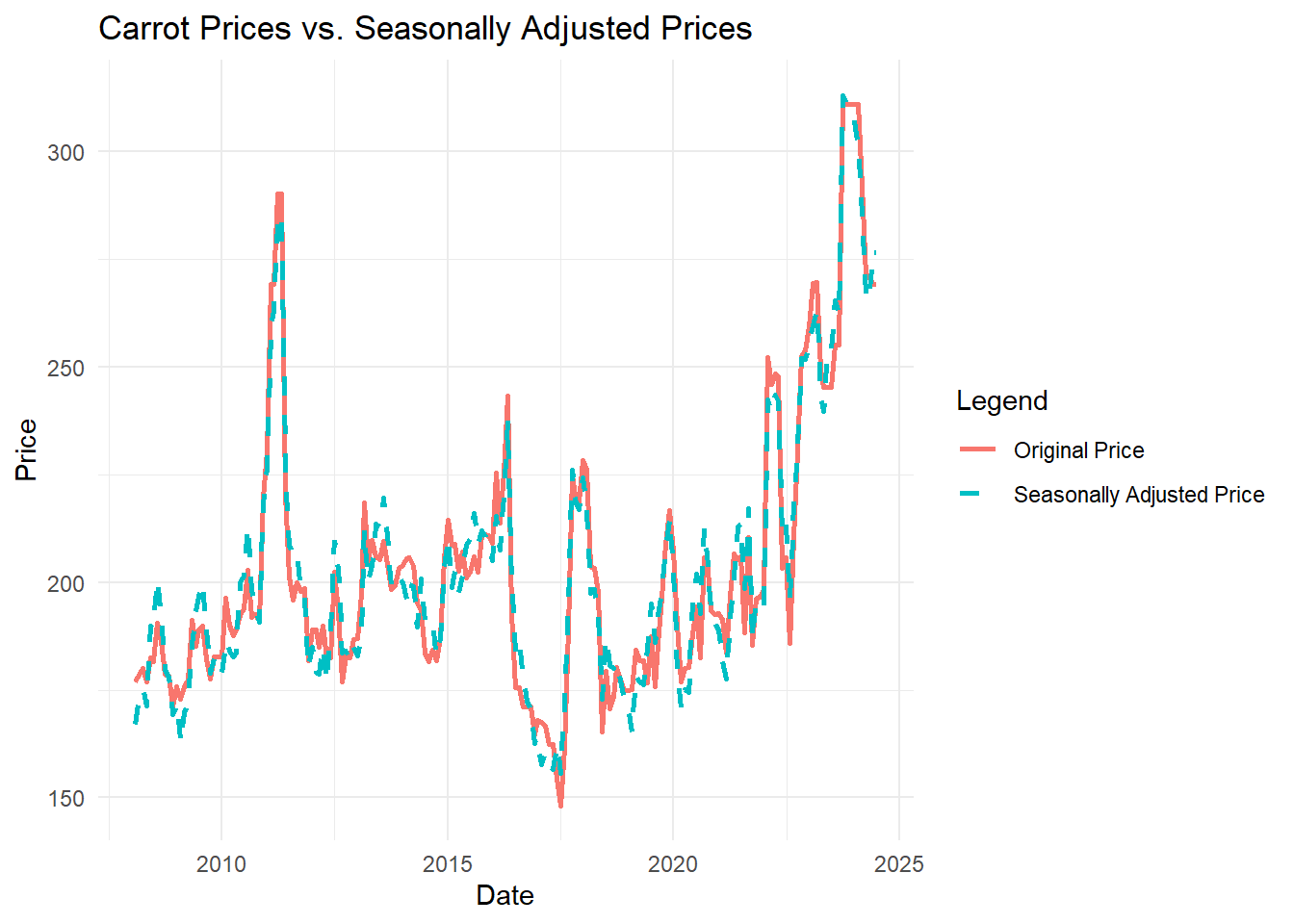

Why Do We Use Seasonally Adjusted Prices?

• Removes regular seasonal patterns to better observe long-term trends.
• Helps in forecasting by isolating the trend and residual components.
• Useful for economic and business analysis, where seasonal cycles might mask underlying changes.

Now, the sa_price column represents the seasonally adjusted price, which can be visualized in Tableau or used in further analysis.

Step 4: Examine the results of the decomposition

Finally, examine the results of the time series decomposition by plotting the decomposed components. The carrot_decomp object contains four components:

1. trend
2. seasonal
3. random
4. figure

You can access each of these components using the $ operator.

To plot the decomposed components, run the following command:

plot(carrot_decomp$trend)
plot(carrot_decomp$seasonal)
plot(carrot_decomp$random)

This will create three separate plots that show the trend, seasonal, and random components of the time series data. You can use these plots to better understand the underlying patterns in your data.

Step 5: Store the Decomposed Data in a Data Frame

To work with the decomposed time series components in further analysis or visualization, we need to store them in a structured dataframe. This allows us to manipulate, export, and integrate the data into other tools like Tableau.

Let’s extract the first four components of the decomposition output and format them into a tidy dataframe:

carrot_decomp_out <- carrot_decomp[1:4] %>% # Extract the first four components of the decomposition output
  as_tibble() %>%            # Convert to a tibble for better readability
  rename(price = x) %>%      # Rename 'x' to 'price' for clarity
  mutate(measure_date = carrot$date,  # Add a measure_date column from the original dataset
         forecast = FALSE) %>%        # Add a column to indicate actual vs. forecasted data
  drop_na()                  # Remove any rows with missing values

How does mutate(measure_date = carrot$date) work without a join?

This works due to positional matching:

• carrot_decomp[1:4] keeps the same row order as carrot_ts, which was built from carrot$price.
• carrot$date retains the original timestamps, allowing direct assignment row by row in mutate().
• Since lengths align, measure_date correctly maps to each observation.

Potential issue: If missing values disrupt alignment, incorrect dates may be assigned. drop_na() helps prevent this.

Check Your Understanding

1. What data type is the variable measure_date in the new data frame?

The data type of measure_date depends on how it was stored in the original dataset (carrot$date). You can check the data type by running:

str(carrot_decomp_out)

If measure_date was originally read in as a character (chr), it will remain a character in the new dataframe. Otherwise, it may already be recognized as a Date object.

2. If measure_date is stored as a character (chr) instead of a date, which function would you use to convert it to a proper date format?

You can use the as.Date() function from base R or either the ymd() function from the lubridate package.

carrot_decomp_out <- carrot_decomp_out %>%
  mutate(measure_date = ymd(measure_date))

If your date format is different (e.g., “MM/DD/YYYY”), use mdy(measure_date) or dmy(measure_date) accordingly.

3. Why is it important to remove missing values drop_na() in time series analysis?

Missing values can disrupt time series analysis and forecasting models, leading to inaccurate results.Many time series functions in R, such as forecast() or decompose(), require complete time series data to function correctly. Removing missing values ensures that the trend, seasonal, and residual components are correctly estimated without gaps in the data.

Recall: Tibbles vs. Data Frames

Go back to the Lab Notes for Week 3 to review the differences between a data frame and a tibble.

R: Forecasting

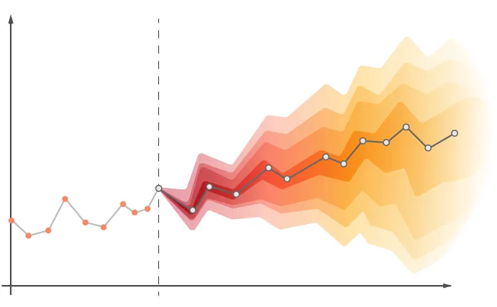
Forecasting allows us to extend our time series into the future by predicting trends, seasonal patterns, and random fluctuations. We will build our forecast by separately modeling the trend, seasonality, and residual (random) components extracted from the decomposition.

Before proceeding with forecasting in R, make sure that the forecast package is loaded.

Step 1: Extract the trend, seasonal, and residual components

The decompose() function breaks a time series into three key components:

1. Trend: The long-term upward or downward movement in the data.
2. Seasonality: The repeating patterns at fixed intervals (e.g., monthly, quarterly).
3. Residual (Random Noise): The part of the time series that is unexplained after removing the trend and seasonality.

We extract these components from the decomposition object using the $ operator and remove any missing values with na.omit().

Understanding na.omit() Syntax

The na.omit() function removes missing values (NAs) from a dataset or vector. This is especially useful in time series analysis, where missing values can interfere with forecasting models.

clean_data <- na.omit(original_data)

• original_data \(\rightarrow\) The vector, dataframe, or time series from which to remove missing values.
• clean_data \(\rightarrow\) The resulting dataset with all NAs removed.

# Extract the trend, seasonal, and residual components
carrot_trend <- na.omit(carrot_decomp$trend) # Extract trend component and remove NAs

carrot_seasonal <- na.omit(carrot_decomp$seasonal)[7:(length(carrot_ts)-6)] %>%
  ts(.,start = c(2008,2), frequency = 12) # Extract and convert seasonality into a time series

carrot_residuals <- na.omit(carrot_decomp$random) # Extract residual component and remove NAs

Why Remove Missing Values?

• Missing values can cause errors in forecasting models that require a continuous time series.
• Functions like forecast() and arima() do not work well with missing values.
• Removing NAs ensures that only complete data is used for trend, seasonal, and residual modeling.

Now that we have extracted and cleaned these components, we are ready to forecast each one separately in the next step.

Step 2: Forecast the trend, seasonal, and residual components

To forecast each component, we use the forecast() function from the forecast package in R.

Understanding forecast() Syntax

The forecast() function is used to generate future values of a time series based on past observations and trends.

forecasted_ts <- forecast(model_or_ts, h = forecast_horizon, level = confidence_interval)

• model_or_ts \(\rightarrow\) A time series object or fitted model (such as ARIMA or ETS) used for forecasting.
• h \(\rightarrow\) The number of future periods to forecast (e.g., h = 12 for 12 months ahead).
• level \(\rightarrow\) The confidence level for the prediction intervals (e.g., level = 95 for 95% confidence intervals).
• forecasted_ts \(\rightarrow\) The resulting forecast object containing predicted values, confidence intervals, and model details.

Forecasting Trend and Seasonal Components

To project future values, we use the forecast() function on the trend and seasonal components separately.

# Forecast the trend component for the next 12 months
carrot_trend_forecast <- forecast(carrot_trend, level = 95, h = 60)
plot(carrot_trend_forecast)

# Forecast the seasonal component for the next 12 months
carrot_seasonal_forecast <- forecast(carrot_seasonal, level = 95, h = 60)
plot(carrot_seasonal_forecast)

Check your output: Did you get a warning? If so, what does the warning message indicate? This may be due to decompose() treating seasonality as a deterministic component, meaning it assumes seasonality repeats exactly. Since there’s no inherent randomness, confidence intervals may not be meaningful.

Forecasting Residuals

The residual component captures the random variation left after accounting for trend and seasonality. Unlike trend and seasonal components, residuals require a statistical model to forecast. One common approach is to use a Moving Average (MA) model.

# Create a time series object for the residuals
carrot_residuals_ts <- ts(carrot_residuals, frequency=12, start = c(2007, 8))

# Fit an MA(1) model to the residuals
carrot_residuals_model <- arima(carrot_residuals_ts, order = c(0,0,1))

# Forecast the residuals for the next 12 months
carrot_residuals_forecast <- forecast(carrot_residuals_model, level = 95, h = 60)

Why do we model the residuals separately? Unlike the trend and seasonal components, the residuals are unpredictable and must be modeled probabilistically rather than simply extended forward.

Understanding arima() Syntax

The arima() function fits an Autoregressive Integrated Moving Average (ARIMA) model to a time series for forecasting.

model <- arima(ts_object, order = c(p, d, q))

• ts_object \(\rightarrow\) The time series data.
• order = c(p, d, q):
  • p (autoregressive order) \(\rightarrow\) Number of lagged observations used as predictors.
  • d (differencing order) \(\rightarrow\) Number of times the data is differenced to make it stationary.
  • q (moving average order) \(\rightarrow\) Number of past forecast errors used in the model.

Example: Fit an ARIMA(1,0,1) model (AR(1) + MA(1)) to a time series:

carrot_arima <- arima(carrot_ts, order = c(1, 0, 1))

This model uses one lagged value and one past error term to make predictions.

This approach ensures that our final forecast accounts for all key components of the time series: trend, seasonality, and random variation.

Step 3: Combine the forecasted components to obtain the final forecast

Now that we have separate forecasts for the trend, seasonal, and residual components, we need to combine them to generate the final forecasted values for the time series.

1. Compute the Final Forecast

The final forecast is the sum of the forecasted trend, seasonal, and residual components.

# Combine the forecasted components to obtain the final forecast
carrot_forecast <- carrot_trend_forecast$mean + 
                    carrot_seasonal_forecast$mean + 
                    carrot_residuals_forecast$mean

View(carrot_forecast)

# Compute upper bound for confidence interval
carrot_forecast_upper <- carrot_trend_forecast$upper + 
                          carrot_seasonal_forecast$upper + 
                          carrot_residuals_forecast$upper

View(carrot_forecast_upper)

# Compute lower bound for confidence interval
carrot_forecast_lower <- carrot_trend_forecast$lower + 
                          carrot_seasonal_forecast$lower + 
                          carrot_residuals_forecast$lower

View(carrot_forecast_lower)

At this point, carrot_forecast contains the predicted future values, while carrot_forecast_upper and carrot_forecast_lower provide confidence intervals around those predictions.

2. Convert Forecasted Values into a Data Frame

Since forecast() returns a special object, we need to convert the results into a standard data frame (a tibble in this case) before merging it with the original dataset.

Important: The date inside as_date() should be set to the first forecasted date, which is the month immediately following your last observed data point. We can code this dynamically.

# Convert forecasted values into a tibble with corresponding dates
max(carrot_decomp_out$measure_date) # Determine the last date of the time series decomposition to determine which was the first forecasted date

carrot_forecast_df <- tibble( # Create a tibble (a modern dataframe in R)
  price = carrot_forecast, # Stores the forecasted price values
  upper = carrot_forecast_upper[,1], # Extracts the upper confidence interval for the forecast
  lower = carrot_forecast_lower[,1] # Extracts the lower confidence interval for the forecast
  ) %>%
  mutate(measure_date = seq(as_date(max(carrot_decomp_out$measure_date)) + months(1), 
                            by = "months", 
                            length.out = nrow(.)))

What This Block of Code Does

• The forecasted values from forecast() are not in a standard tabular format, so we need to reshape them.
• We assign a corresponding date (measure_date) to each forecasted value, ensuring alignment with the original time series.
• The confidence intervals (upper and lower) allow us to quantify forecast uncertainty.

Why is [,1] used in carrot_forecast_upper[,1] and carrot_forecast_lower[,1]?

The forecast() function returns confidence intervals as matrices, with each column representing different confidence levels (e.g., 80%, 95%).

However, if only one confidence level is specified in forecast(), the matrix will only contain one column.

Breakdown:

• forecast_object$upper and forecast_object$lower are matrices, not vectors.
• If one confidence level is specified (e.g., level = 95), the matrix will have only one column, and [,1] is required to extract the values.
• If multiple confidence levels are specified (e.g., level = c(80, 95)), the matrix will have two columns, where [,1] corresponds to the 80% interval and [,2] corresponds to the 95% interval.

Example using carrot_forecast:

# Forecasting with a single confidence level (e.g., 95%)
carrot_trend_forecast <- forecast(carrot_trend, level = 95, h = 60)

# Check the structure of the confidence interval matrix
dim(carrot_trend_forecast$upper)  # Output: [1:60, 1] → 60 time steps, 1 confidence level

# Extract the only available confidence interval
carrot_forecast_upper <- carrot_trend_forecast$upper[,1]  
carrot_forecast_lower <- carrot_trend_forecast$lower[,1]

In this case, because we only specified one confidence level (level = 95), the output matrix has only one column, and [,1] is needed to extract the values.

If we had specified multiple levels (level = c(80, 95)), we would need to use [,2] to extract the 95% confidence interval.

At this stage, we have a clean forecast dataset that is ready to be appended to the existing observed data. The next step is to merge this with the original time series data and prepare it for visualization in Tableau.

Step 4: Merge Forecasted Data with Observed Data

Now that we have created our forecasted values, we need to append them to the original dataset. However, there is a slight complication:

• Some of the original observed data overlaps with the beginning of the forecasted period.
• This occurs because some data points were lost during the decomposition process (e.g., due to moving averages used in decompose()).
• We have three options for handling this overlap:
  1. Keep both the forecasted and observed data.
  2. Keep only the forecasted values in the overlapping period.
  3. Keep only the observed values in the overlapping period.

For this analysis, we will follow option #3 (keep only the observed values in the overlapping period) and append the remaining forecasted values to the dataset.

# Keep only forecasted data that occurs after the last observed date
carrot_forecast_df <- carrot_forecast_df %>%
  filter(measure_date > max(carrot_decomp_out$measure_date)) %>%
  mutate(forecast = TRUE) # Mark these as forecasted values

# Append forecasted data to the original dataset
final_out <- bind_rows(carrot_decomp_out,carrot_forecast_df)

Step 5: Export Data for Tableau

To prepare for visualization in Tableau, we need to export the final dataset as a CSV file.

# Save the final dataset as a CSV file
write_csv(final_out,"carrot_forecast.csv")

This CSV file will contain:

• Original observed prices
• Decomposed trend, seasonality, and residual components
• Forecasted values for future months
• A forecast indicator column to distinguish real vs. predicted data

Lab Script for Week 6: Time Series Decomposition and Forecasting

# This is the script for lab 06.

setwd("Set your working directory")

# Comment out the following line if you have already installed the forecast package.
install.packages("forecast")


# Load necessary libraries
library(tidyquant)
library(dplyr)
library(tidyr)
library(readr)
library(ggplot2)
library(lubridate)
library(forecast)

# Part 1: Time Series Decomposition

# Retrieve time series data for carrots
carrot <- tq_get(c("WPU01130212"),
                 get = "economic.data",
                 from = "2007-08-01")

# Convert data into a time series object
carrot_ts <- ts(carrot$price,
                start = c(2007,8),
                frequency = 12)

# Decompose the time series
carrot_decomp <- decompose(carrot_ts)

# Compute seasonally adjusted price
carrot_sa_price <- carrot_ts - carrot_decomp$seasonal

# Convert to a tibble for easier handling
carrot_decomp_sa <- tibble(
  measure_date = carrot$date,
  price = carrot$price,
  trend = carrot_decomp$trend,
  seasonal = carrot_decomp$seasonal,
  residual = carrot_decomp$random,
  sa_price = as.numeric(carrot_sa_price) # Seasonally adjusted price converted to numeric for plotting
) %>%
  drop_na()

# Plot original prices vs. seasonally adjusted prices
sa_plot <- ggplot(carrot_decomp_sa, aes(x = measure_date)) +
  geom_line(aes(y = price, color = "Original Price"), size = 1) +
  geom_line(aes(y = sa_price, color = "Seasonally Adjusted Price"), linewidth = 1, linetype = "dashed") +
  labs(title = "Carrot Prices vs. Seasonally Adjusted Prices",
       x = "Date", y = "Price",
       color = "Legend") +
  theme_minimal()

print(sa_plot)

# Plot decomposed components
plot(carrot_decomp$trend)
plot(carrot_decomp$seasonal)
plot(carrot_decomp$random)

# Store decomposition results into a dataframe
carrot_decomp_out <- carrot_decomp[1:4] %>%
  as_tibble() %>%
  rename(price = x) %>%
  mutate(measure_date = carrot$date,
         forecast = FALSE) %>%
  drop_na()

# Part 2: Forecasting

# Extract trend, seasonal, and residual components
which(is.na(carrot_decomp$trend)) # Determine which values are missing
carrot_trend <- na.omit(carrot_decomp$trend)

which(is.na(carrot_decomp$seasonal))
carrot_seasonal <- na.omit(carrot_decomp$seasonal)[7:(length(carrot_ts) - 6)] %>%
  ts(., start = c(2008, 2), frequency = 12)

which(is.na(carrot_decomp$residuals)) # Determine which values are missing
carrot_residuals <- na.omit(carrot_decomp$random)

# Forecast trend and seasonal components
carrot_trend_forecast <- forecast(carrot_trend, level = 95, h = 60)
plot(carrot_trend_forecast)

carrot_seasonal_forecast <- forecast(carrot_seasonal, level = 95, h = 60)
plot(carrot_seasonal_forecast)

# Fit an MA(1) model for residuals and forecast
carrot_residuals_ts <- ts(carrot_residuals, frequency = 12, start = c(2007, 8))
carrot_residuals_model <- arima(carrot_residuals_ts, order = c(0,0,1))
carrot_residuals_forecast <- forecast(carrot_residuals_model, level = 95, h = 60)

# Combine forecasted components
carrot_forecast <- carrot_trend_forecast$mean + 
  carrot_seasonal_forecast$mean + 
  carrot_residuals_forecast$mean

View(carrot_forecast)

carrot_forecast_upper <- carrot_trend_forecast$upper + 
  carrot_seasonal_forecast$upper + 
  carrot_residuals_forecast$upper

View(carrot_forecast_upper)

carrot_forecast_lower <- carrot_trend_forecast$lower + 
  carrot_seasonal_forecast$lower + 
  carrot_residuals_forecast$lower

View(carrot_forecast_lower)

# Convert forecasted values into a tibble with corresponding dates
max(carrot_decomp_out$measure_date) # Determine the last date of the time series decomposition to determine which was the first forecasted date

carrot_forecast_df <- tibble( # Create a tibble (a modern dataframe in R)
  price = carrot_forecast, # Stores the forecasted price values
  upper = carrot_forecast_upper[,1], # Extracts the upper confidence interval for the forecast
  lower = carrot_forecast_lower[,1] # Extracts the lower confidence interval for the forecast
  ) %>%
  mutate(measure_date = seq(as_date(max(carrot_decomp_out$measure_date)) + months(1), 
                            by = "months", 
                            length.out = nrow(.)))

View(carrot_forecast_df)

# Keep only forecasted data that occurs after the last observed date
carrot_forecast_df <- carrot_forecast_df %>%
  filter(measure_date > max(carrot_decomp_out$measure_date)) %>%
  mutate(forecast = TRUE) # Mark these as forecasted values

# Append forecasted data to the original dataset
final_out <- bind_rows(carrot_decomp_out,carrot_forecast_df)

View(final_out)

# Save the final dataset as a CSV file
write_csv(final_out,"carrot_forecast.csv")

Tableau

Now we will use Tableau to visualize the forecasted time series and its decomposed components from R using carrot_forecast.csv.

Step 1: Connect Your Data in Tableau

1. Open Tableau and connect to the CSV file you exported from R (carrot_forecast.csv).
   • This file contains:
     • Observed carrot prices (price)
     • Forecasted values (forecast)
     • Three decomposition components (trend, seasonality, random)
2. Make sure the fields are correctly formatted in Tableau. If necessary, change the data types so each variable is formatted correctly:
   • measure_date = Date
   • price, seasonal, trend, random, upper, lower = Number (decimal)
   • forecast = Boolean

Note

If you are working with multiple time series data, filter the measure_date field so that all worksheets begin at the relevant start date for your analysis.

Step 2: Visualizing Time Series Decomposition

In Sheet 1:

1. Plot the raw price data as a line chart.
   • Add price to the row shelf. Display as AVG(Price).
   • Add measure_date to the column shelf. Display measure_date as Measure > MONTH().
2. Make sure forecasted values (forecast = TRUE) are filtered out when generating the line graph.
   • Drag forecast to the Filters card. Check the box next to True. Click OK.
3. Add the trend, seasonal, and random components as new panes below the price line.
   • Add trend to the row shelf. Display as AVG(Trend).
   • Add seasonal to the row shelf. Display as AVG(Seasonal).
   • Add random to the row shelf. Display as AVG(Random).
4. Experiment with Tableau’s built-in smoothing:
   • Convert the raw price data to a moving average using Quick Table Calculation.
     
   • Compare Tableau’s moving average to the one calculated in R.
5. Add a caption answering the following questions:
   • What are the overall trends in the data?
     
   • Which seasons have higher or lower prices?
     
   • How much variation remains unexplained after removing trend and seasonality?

Step 3: Forecasting in Tableau

In Sheet 2:

1. Create a new calculated field called observed_price.
   • IF [Forecast]=FALSE THEN [Price] ELSE NULL END
2. Plot the observed prices as a line chart.
   • Add measure_date to the column shelf. Display measure_date as Measure > MONTH().
   • Add observed_price to the row shelf. Display as AVG(observed_price).
   • Drag forecast to the Filters card. Check the box next to True. Click OK.
3. Create a forecast in Tableau.
   • Switch to the Analytics tab from the Data tab. In the Analytics tab, there is a Forecast option under the Model section.
   • To add a forecast to this plot, hold the Forecast option and drag it on to the scatter plot (or visualization area). You will see that it gives us one option that we can add to our graph.
   • To change the forecast, right click on the confidence interval around the forecasted values. Select Forecast > Forecast Options…
   • What do you notice?

Step 4: Compare Tableau’s forecast with R’s forecast

In Sheet 3:

1. Plot the raw price data as a line chart.

   • Add price to the row shelf. Display as AVG(Price).
   • Add measure_date to the column shelf. Display measure_date as Measure > MONTH().

2. Drag forecast to the Color Marks Card.

3. Plot the upper and lower bounds of the confidence interval of the forecasted values.

   • Add upper to the row shelf. Display as AVG(upper).
   • Right click upper and select Dual Axis.
   • Hover over the secondary axis that corresponds with Avg. Upper. Right click it. Select Synchronize Axis.
   • Drag lower to the secondary axis. You will need to reset the axis.
   • Hover over the axis that corresponds with Avg. Upper. Right click it. Select Synchronize Axis.
   • Now you will see all lines: observed prices, forecasted prices, the upper bound, the lower bound.

4. Create a new dashboard that combines both forecasts:

   • The forecast generated in R (forecast = TRUE)
   • The forecast generated in Tableau

5. Add a text box to explain forecast differences:

   • Why do the R and Tableau forecasts differ?
     
   • Which model appears more accurate?
     
   • How does seasonality impact the predictions?

6. Hide unnecessary worksheets:

   • Right-click the worksheet tab → Select Hide.

Step 5: Identifying Seasonal Trends

1. Create a dashboard to analyze seasonal trends.
   • Compare price patterns by month (as we did in Step 2) vs. quarter. Go through the same process as we did for Step 2, but display measure_date as Measure > QUARTER().
2. Add a text box describing important takeaways:
   • Are trends more apparent when comparing months vs. quarters?
     
   • Are there notable differences in annual trends within a given month or quarter?

Final Step: Publish to Tableau Public

1. Format your workbook following the guidelines for effective visualizations:
   • Add color, titles, and labels to improve readability.
     
   • Make sure that all charts effectively communicate your insights.
2. Publish your workbook to Tableau Public. Your workbook should include:
   • One worksheet (Step 2 - Time Series Decomposition from R)
     
   • Two dashboards (Step 3 - Forecasting & Step 4 - Seasonal Trends)