Week 11:
Data Analysis in Practice

Motivation

Our goal in this course is to teach tools and processes for analyzing data to inform decision-making.

You now have some tools for data analysis.

Today, let’s revisit the process.

How do we get from question to answer?

Agenda

Finding patterns in convenience store sales

Project 2: Q&A

Project Context

Who am I?

I’m a researcher interested in store-level variation in product offerings, consumer behavior, and store performance across the U.S. convenience store sector.

I focus on how retail format, customer base, and product mix interact across locations.

Who are you?

Scenario: A supplier of packaged snacks or beverages wants to know which types of stores would be best targets for a new product line.

What is my research question?

Can we identify meaningful segments of convenience stores based on transaction-level data?

This leads to sub-questions like:

Are there distinguishable store clusters based on number of customers, product diversity, and fuel share?
How do consumer shopping patterns vary across those clusters?
How are clusters positioned across the United States?

Why does it matter?

Understanding store segments helps us:

Identify business strategies that different store types pursue (e.g., fuel-heavy vs. product-diverse)
Highlight variation in access to different products, which matters for consumer choice
Support targeted business decisions, like vendor partnerships or tailored promotions
Potentially link to spatial inequities in access to goods and services

How do I answer it?

I use a cluster analysis of national convenience store data:

Data: Transaction-level data linked to store and product characteristics
Variables: Total sales, unique customers, product diversity, fuel share, and chain size
Method: K-means clustering on log-transformed and scaled variables
Interpretation: Examine features of each cluster to understand differences in store types

EDA (Cluster Analysis)

Read In Data

# Read in the shopper_info dataset
# This dataset contains detailed information on shoppers and their transactions for July 2023
shopper_info <- read_csv("https://csu-arec-330.github.io/materials/unit_02/inputs/shopper_info.csv")

# Separate data file with shopper ID and their zipcode
shopper_zip <- read_csv("https://csu-arec-330.github.io/materials/unit_02/inputs/shopper_zip.csv")

# Read in the GTIN dataset
# This file links products to their Global Trade Item Numbers, akin to SKUs or UPCs
gtin <- read_csv("https://csu-arec-330.github.io/materials/unit_02/inputs/gtin.csv")

# Read in the store_info dataset
# Contains details about each store, linkable to shopper_info via store_id
store_info <- read_csv("https://csu-arec-330.github.io/materials/unit_02/inputs/store_info.csv")

Clean the Data

# Join the data frames together
store_shopper_gtin_left <- left_join(store_info, shopper_info, by = "store_id") %>%
  left_join(gtin, by = "gtin")

# Look at the raw count of observations after join
total_observations <- nrow(store_shopper_gtin_left)
print(paste0("Total observations of raw data: ", total_observations))

[1] "Total observations of raw data: 161906"

# Look at the number of distinct store id's prior to cleaning the data
store_count_raw <- length(unique(store_shopper_gtin_left$store_id))
print(paste0("Count of distinct stores in raw data: ", store_count_raw))

[1] "Count of distinct stores in raw data: 23570"

# Clean and transform the raw data
clean_data <- store_shopper_gtin_left %>%

    # Remove observations with negative or zero unit price (e.g., returns or invalid entries)
  filter(unit_price > 0) %>% 
  
  # Remove observations of stores missing shopper IDs
  filter(!is.na(shopper_id)) %>%
  
  # Calculate total spending per line item
  mutate(total = unit_price * unit_quantity) %>%
  
  # Convert transaction_set_id and transaction_item_id to integers without decimals
  mutate(transaction_set_id = format(transaction_set_id, scientific = FALSE, trim = TRUE), 
         transaction_item_id = format(transaction_item_id, scientific = FALSE, trim = TRUE)) %>%
  
  # Arrange data by store_id and zip_code
  arrange(store_id, zip_code)

What is my Unit of Analysis?

# Check how many distinct shoppers are in the clean dataset
unit_of_analysis <- length(unique(clean_data$store_id))
print(paste0("Unit of analysis (store-level): ", unit_of_analysis))

[1] "Unit of analysis (store-level): 6750"

Cluster Analysis Setup

I want to analyze stores using:

Unique customers
Total sales
Product diversity
Fuel share
Chain size

I need to summarize these metrics to the store-level as this is my unit of analysis.

# Summarize metrics at the store level
store_summary <- clean_data %>%
  group_by(store_id) %>%
  summarise(
    total_sales = sum(unit_price * unit_quantity, na.rm = TRUE),               # Total revenue
    unique_customers = n_distinct(shopper_id),                                 # Number of unique customers
    product_diversity = n_distinct(gtin),                                      # Number of unique products sold
    fuel_transactions = sum(is.na(gtin) | gtin == 0),                          # Number of fuel transactions
    total_transactions = n_distinct(transaction_set_id),                       # Total number of transactions
    fuel_share = fuel_transactions / total_transactions,                       # Fuel share of transactions
    .groups = "drop"
  ) %>%
  left_join(store_info %>% select(store_id, chain_size), by = "store_id") %>%      # Add chain size
  filter(!is.na(chain_size))

# Final dataset: merge summaries if desired
final_dataset <- store_summary %>%
  left_join(store_info %>% select(-chain_size), by = c("store_id")) %>%
  arrange(store_id, zip_code)

Summary Stats

sumstats <- store_summary %>%
  summarise(
    mean_sales = mean(total_sales),
    mean_customers = mean(unique_customers),
    mean_products = mean(product_diversity),
    mean_fuel_share = mean(fuel_share),
    mean_chain_size = mean(chain_size),
    .groups = "drop"
  )

print(sumstats, n = Inf, width = Inf)

# A tibble: 1 × 5
  mean_sales mean_customers mean_products mean_fuel_share mean_chain_size
       <dbl>          <dbl>         <dbl>           <dbl>           <dbl>
1       858.           4.21          3.19           0.809            40.3

Log-Transformations

Because these variables are very skewed, I log-transform unique_customers, total_sales, product_diversity, and chain_size.

# I noticed that the distribution of my store attributes is very skewed, so I want to rescale them.
final_dataset <- final_dataset %>%
  mutate(
    log_customers = log(unique_customers + 1),
    log_sales = log(total_sales + 1),
    log_products = log(product_diversity + 1),
    log_chain_size = log(chain_size + 1)
  )

GGPairs Plot

# Run the ggpairs() command
final_dataset %>%
  select(log_customers, log_sales, log_products, fuel_share, log_chain_size) %>% 
  ggpairs()

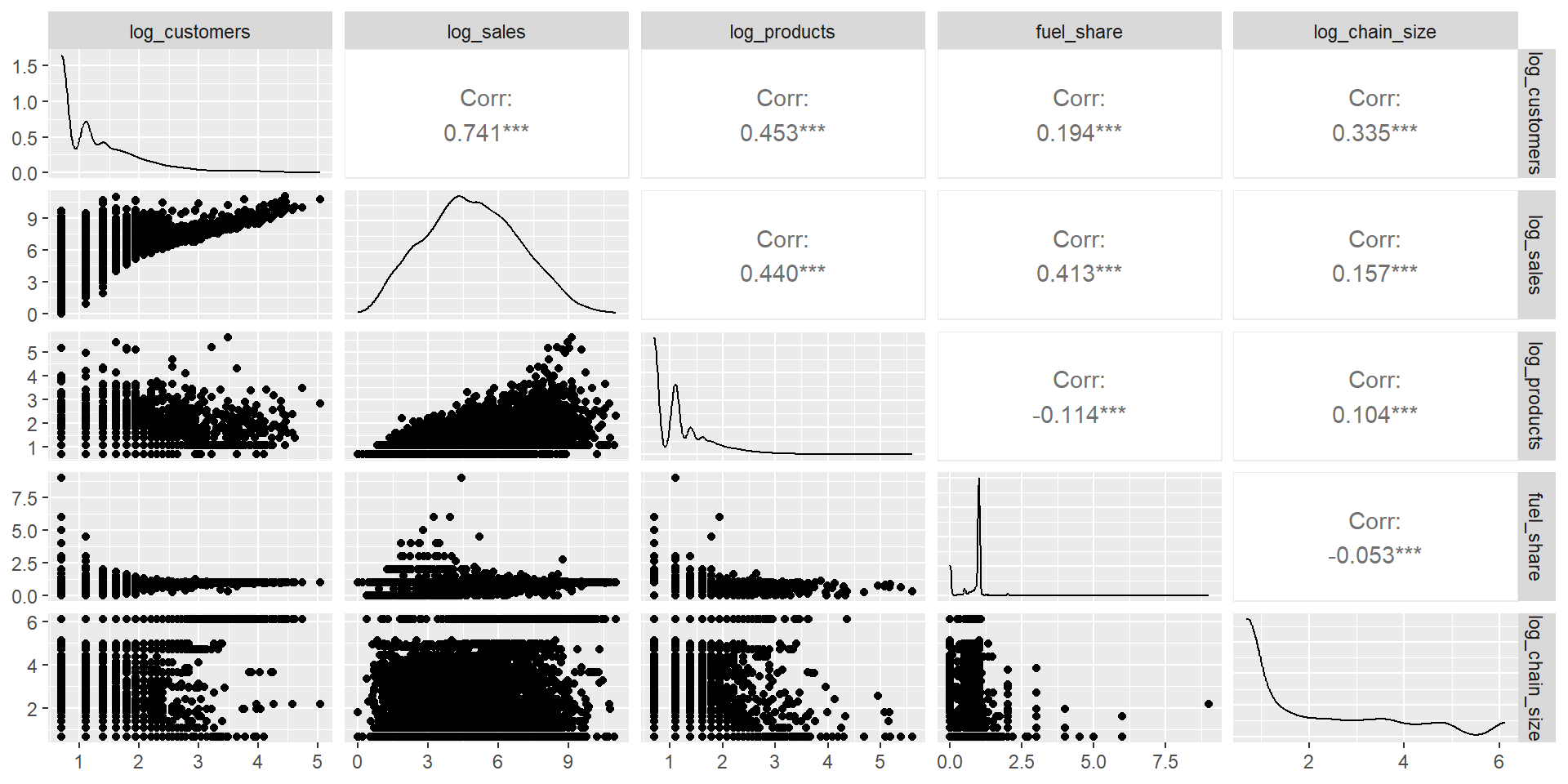
Almost there… Need to rescale variables

# Prepare data for clustering
cluster_data <- final_dataset %>%
  select(log_customers, log_sales, log_products, fuel_share, log_chain_size)

cluster_scaled <- scale(cluster_data)

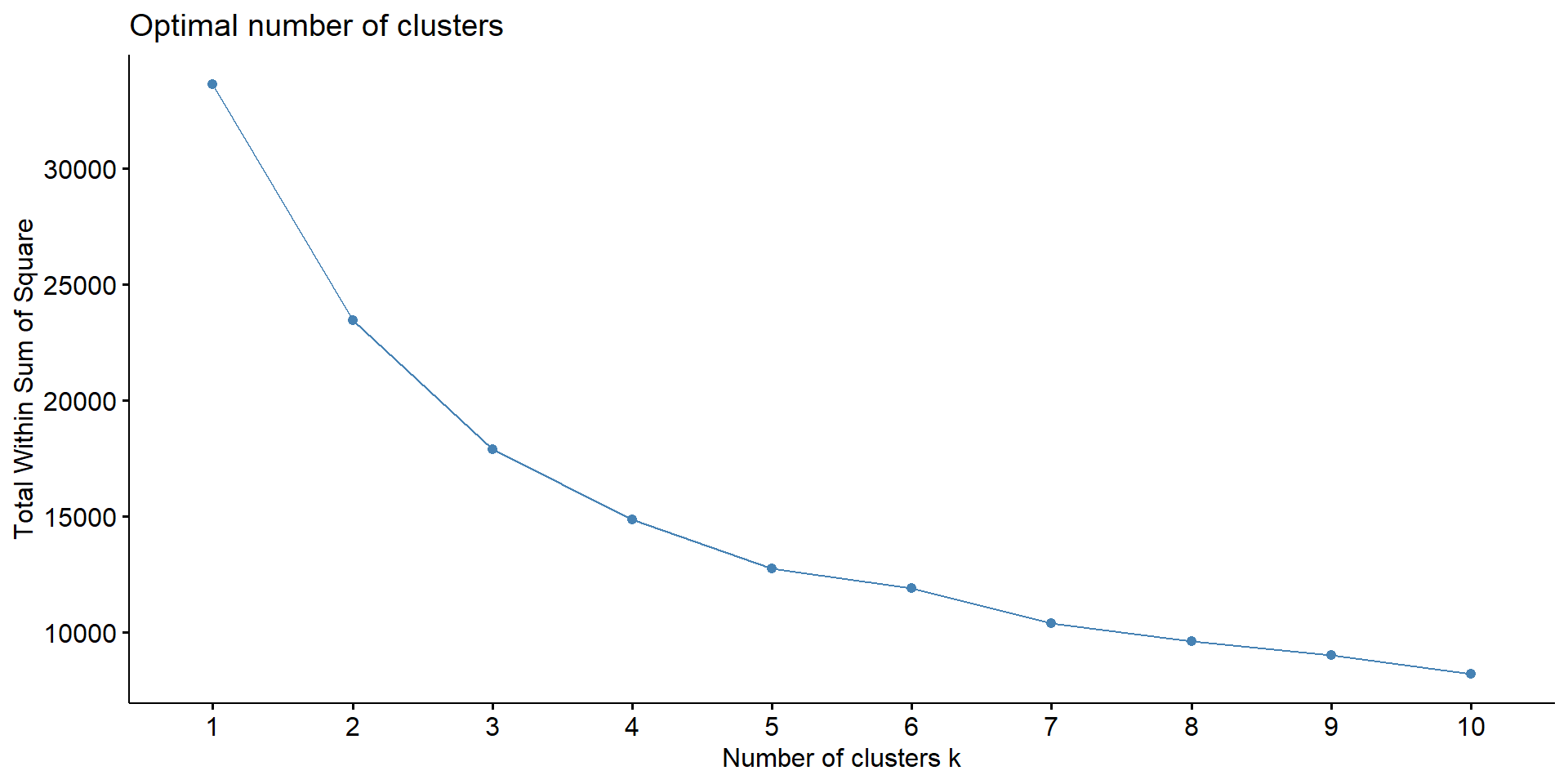
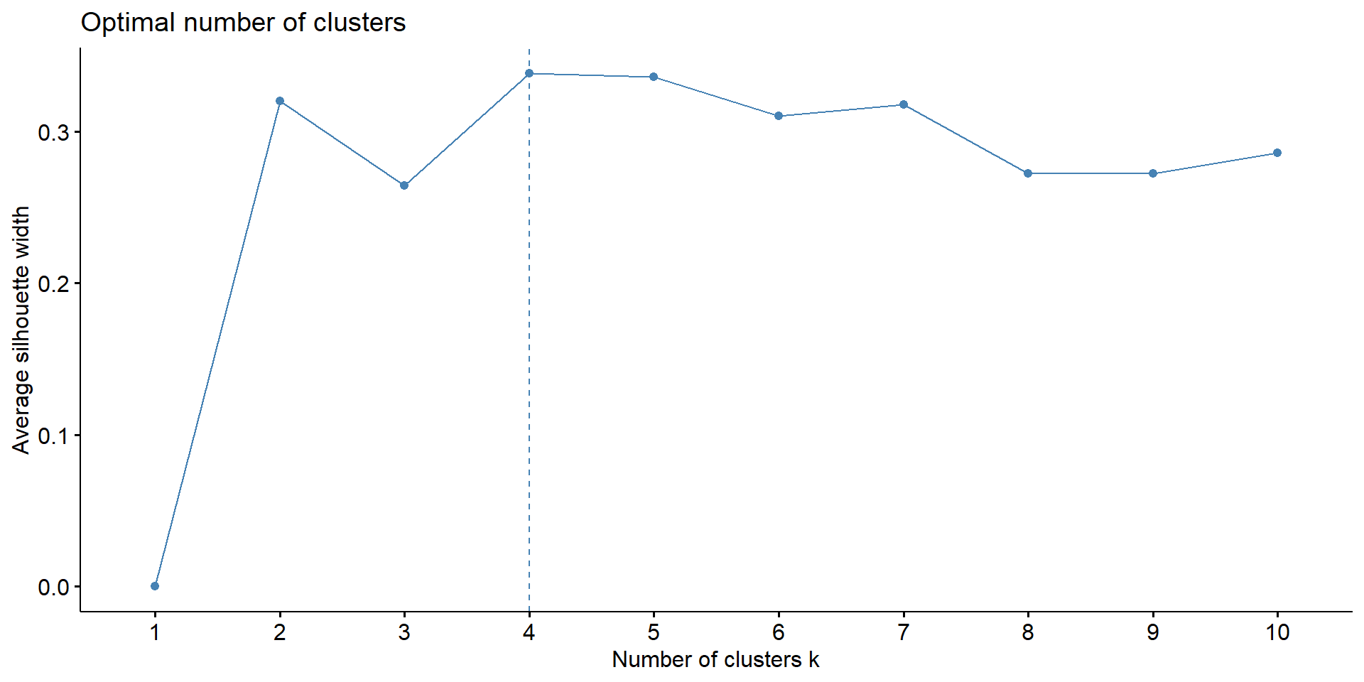
Choosing the Number of Clusters

# Use two common methods to help choose the number of clusters.

# Elbow Method
fviz_nbclust(cluster_scaled, kmeans, method = "wss")

# Silhouette Method
fviz_nbclust(cluster_scaled, kmeans, method = "silhouette")

Perform Clustering and Add to Data

# Perform k-means clustering on logged and scaled data
set.seed(123)
kmeans_fit <- kmeans(cluster_scaled, centers = 4, nstart = 25)

# Add cluster to dataset
final_dataset$cluster <- factor(kmeans_fit$cluster)

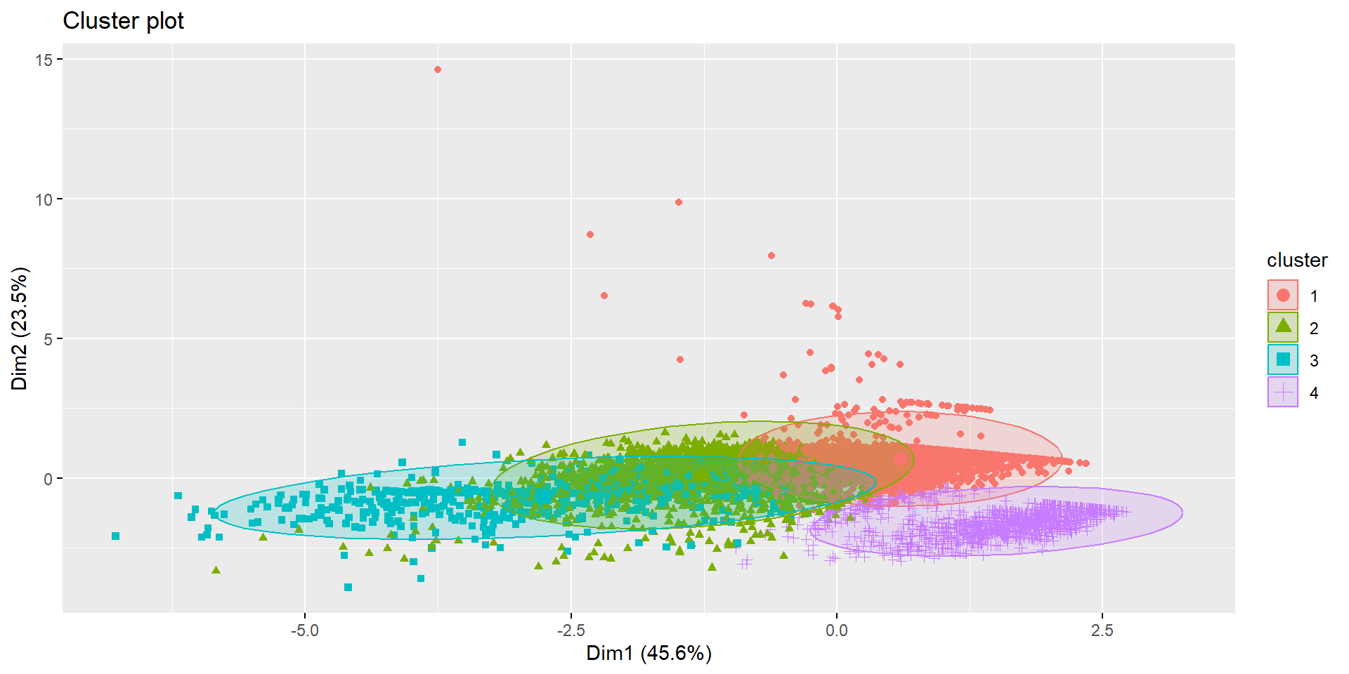
Visualizing the Clusters

fviz_cluster(kmeans_fit, data = cluster_scaled, geom = "point", ellipse.type = "norm")

Compare Cluster Averages

# Use the original (non-logged) variables because you're summarizing actual store characteristics — not the transformed versions.
final_clusters <- final_dataset %>%
  group_by(cluster) %>%
  summarize(across(c(unique_customers, total_sales, product_diversity, fuel_share, chain_size), mean))

print(final_clusters)

# A tibble: 4 × 6
  cluster unique_customers total_sales product_diversity fuel_share chain_size
  <fct>              <dbl>       <dbl>             <dbl>      <dbl>      <dbl>
1 1                   1.63       163.               1.36     1.03        16.0 
2 2                   5.53      1796.               6.81     0.894        5.82
3 3                  19.8       3642.               4.78     0.942      279.  
4 4                   1.25        17.9              2.38     0.0648      27.4

Most Frequent City by Cluster

What are the top 5 cities where stores of each cluster are located?

final_dataset %>%
  select(cluster, city) %>%
  group_by(cluster, city) %>%
  summarize(n = n(), .groups = "drop") %>%
  group_by(cluster) %>%
  slice_max(order_by = n, n = 5) %>%
  ungroup() %>%
  kable()

cluster	city	n
1	Houston	22
1	Milwaukee	19
1	Nashville	19
1	Canton	16
1	Louisville	16
2	Pittsburgh	13
2	Dayton	9
2	Raleigh	9
2	Charlotte	8
2	Livonia	8
2	Taylor	8
3	Raleigh	28
3	Abilene	18
3	Carlsbad	12
3	Hobbs	12
3	Clovis	11
3	Roswell	11
4	Omaha	13
4	Houston	10
4	Charleston	6
4	Columbia	6
4	Salem	6

Cluster 1: Fuel-Dominant, Low-Volume Stores

These stores are primarily fuel-oriented, with minimal in-store shopping. Likely located in rural or highway areas.

Very few customers (~1.63)
Low sales (~$163)
Very limited product variety (~1.36)
Fuel share > 1 (likely a data artifact, possibly due to fuel-only transactions dominating the count)

Mid-Volume, High-Diversity Stores

These stores show a more balanced customer base and diverse product offerings, suggesting a hybrid model of fuel + general merchandise.

Moderate customers (~5.53)
Strong sales (~$1,796)
High product diversity (~6.81)
High fuel share (~89%)

Cluster 3: High-Volume, High-Sales Stores

These stores are top performers in both customer traffic and revenue. Possibly urban or destination stores with strong retail and fuel performance.

Most customers (~19.79)
Highest sales (~$3,641)
Moderately high product diversity (~4.78)
High fuel share (~94%)

Cluster 4: Low-Volume, Non-Fuel Stores

These appear to be underperforming stores with limited traffic, low sales, and minimal fuel activity. May represent struggling or niche-format stores.

Fewest customers (~1.25)
Lowest sales (~$17.90)
Low product diversity (~2.38)
Very low fuel share (~6.5%)

Revisiting the Research Question

Can we identify meaningful segments of convenience stores based on transaction-level data?

Answer: Yes!

The clusters suggest four distinct operational models among stores in the dataset.
These segments differ in customer base, sales volume, product assortment, and fuel reliance — reflecting meaningful variation in store strategy and performance.

Why it matters:

Product suppliers may target Clusters 2 and 3 with expanded assortments or promotions.
Clusters 1 and 4 may signal opportunities for format innovation, operational improvement, or market exit.
Retailers can use this segmentation to prioritize investments, tailor inventory strategies, and benchmark performance.

Project 2: Q&A

Break into groups

Based on your initial cluster analysis:

What are some effective ways to present summary statistics and visualize your data?
How do the results of the clustering analysis inform your research question?
What insights can you take away from your analysis? What story does it tell?

Summarizing Data and Visualizing Patterns

What are some effective ways to present summary statistics and visualize your data?
- Scatterplots, histograms, maps
- Descriptive statistics (mean, standard deviation, range)
How can you highlight geographical differences in your variables?
- Choropleth maps, bubble maps
What other visualizations or techniques could be useful for your specific project?

Conducting Cluster Analysis

What is your rationale for using cluster analysis to answer your research question?
- Identifying groups or segments with similar characteristics
- Exploring patterns and relationships in the data
How will you choose the appropriate variables for clustering?
- Relevant to your research question
- Capturing different aspects of the data (e.g., demographics, economic factors)
What are some potential challenges or limitations of your cluster analysis?
- Choosing the right number of clusters
- Interpreting and validating the clusters

Communicating Cluster Analysis

What story does your cluster analysis tell?
- “Sales in segment x are strong.”
Create visuals to support your story
- Bar chart with sales by segment
What is your call to action?
- “We should market segment x.”

Summary

Summarizing data and visualizing patterns
Conducting cluster analysis
Communicating cluster analysis

Week 11: Data Analysis in Practice

Motivation

Agenda

Project Context

Who am I?

Who are you?

What is my research question?

Why does it matter?

How do I answer it?

EDA (Cluster Analysis)

Read In Data

Clean the Data

What is my Unit of Analysis?

Cluster Analysis Setup

Summary Stats

Log-Transformations

GGPairs Plot

Almost there… Need to rescale variables

Choosing the Number of Clusters

Perform Clustering and Add to Data

Visualizing the Clusters

Compare Cluster Averages

Most Frequent City by Cluster

Cluster 1: Fuel-Dominant, Low-Volume Stores

Mid-Volume, High-Diversity Stores

Cluster 3: High-Volume, High-Sales Stores

Cluster 4: Low-Volume, Non-Fuel Stores

Revisiting the Research Question

Project 2: Q&A

Break into groups

Summarizing Data and Visualizing Patterns

Conducting Cluster Analysis

Communicating Cluster Analysis

Summary

Week 11:
Data Analysis in Practice