Week 13 Lab: Introduction to Panel Data Analysis and Spatial Data in R

This Lab Contributes to Course Objectives: 1, 3, 4, 5, 7, 8

Learning Objectives R

• Read in and manipulate spatial data in R

• Join spatial data

• Prepare data for mapping in Tableau

• Prepare data for regression analysis

Introduction to Spatial Data in R

Spatial data is a form of cross-sectional data that contains geographic information.¹ Examples include the location of a store or park, the boundary of a parcel of land, or the location of a weather measurement. In many cases, we need to process that data in some way or join it to other (potentially spatial) data for analysis.

Spatial Data Formats

Two common types of spatial data in R are vector and raster data.

• Vector data represent geographic features as points, lines, and polygons. Vector data is often used to represent discrete features such as the boundaries of a city or the location of a specific point of interest. It is common to find data with specific location information (e.g., latitude and longitude coordinates).

• Raster data represent geographic features as a grid of cells with values assigned to each cell. Raster data, on the other hand, is often used to represent phenomena such as elevation or temperature that are continuous across the landscape.

R Packages

Working with spatial data in R involves using specialized packages and functions to read, manipulate, and visualize the data. Some popular packages for working with spatial data in R include sf and raster. With these tools, it’s possible to perform a wide range of spatial analyses, such as overlaying different layers of data to find areas of overlap or proximity, extracting data for specific regions of interest, and creating custom maps and visualizations. Taro Meino has written a useful reference on using R for GIS.

Objective

We will develop a spatial dataset in which you join convenience store location data with county level data from the U.S. Census and weather data from NOAA.

Unit of Analysis

Always be paying attention to what is your unit of analysis or unit of observation. In this lab, our unit of analysis is the county, so we need to associate each convenience store with a county.

Setup

Our first step is to start an R script and load packages.

# This is the R script for Week 13 Lab. 
# This script will demonstrate how to work with spatial data and conduct some basic operations (e.g., intersection)

setwd("set my working directory")
getwd() # Confirm I am in the proper working directory.

# load packages
library(pacman)
p_load(tidyverse,janitor,sf,tigris,mapview,tidycensus,dplyr)

# Read in convenience store location dataset
store_raw <- read_csv("https://csu-arec-330.github.io/materials/unit_03/inputs/store_info.csv.gz")

Converting Data to a Spatial Format

The field of geography and geographic information systems (GIS) specialize in understanding and working with geospatial data. Locations are known because of a commonly understood reference system called a Coordinate Reference System (CRS). Think about a graph with \(x\) and \(y\) dimensions. A point on that graph has a set of coordinates that tell you the location. CRS in GIS can be more complicated because we are thinking about points that exist on a globe (this would be easier if the earth were flat).

The store_raw dataframe has latitude and longitude coordinates. At this point, R considers these numbers like any other numeric variable. There are packages built to understand and work with geospatial data. sf stands for simple features and is a commonly used package. We will use it to convert the store_raw data into a spatially aware data frame.

# Convert data frame to a points simple feature object
store_geo <- store_raw %>%
  
  # First, we subset the variables `store_id` and the coordinates.
  select(store_id, latitude, longitude) %>% 
  
  # Tells R that these are essentially $x$ and $y$ coordinates in a certain projection (represented by the code 4326). See <https://epsg.io/> for more information.
  st_as_sf(coords=c("longitude","latitude"), crs = st_crs(4326))  

Result: store_geo is a different object than we have worked with before but it looks and behaves like a familiar dataframe. You can mutate new variables, arrange, and even summarize, but summarize also performs geospatial operations because you are changing the unit of analysis.

It is often helpful to look at data especially when mapping. R can leverage very powerful mapping tools, but we will just use them to make sure we are doing what we think we are doing. We can use mapview() to look at the data.

# Configure mapview to render points directly in the RStudio Viewer (not using flatgeobuf)
mapviewOptions(fgb = FALSE)

# Display the store locations as an interactive map
mapview(store_geo)

After you plot these points, what do you observe about the locations of the stores? What might you want to do with your data to remove outliers? Consider these answers as we move into the next section.

Getting Census Boundaries

The dataframe store_raw contains a lot of meta information but not county.

Boundaries for commonly used geometries (such as county boundaries) are available from the US Census and accessible through an API to the Census repository of these boundaries (called Tiger). The R package tigris provides a very convenient API to access them.

# Fetch data for county polygons using the 'tigris' package
us_co <- tigris::counties(cb = TRUE, class = "sf") %>%
  
  # Clean column names to snake_case using janitor
  janitor::clean_names() %>%
  
  # Convert land area from square meters to square miles
  mutate(aland = aland / 2.59e+6) %>%
  
  # Transform the coordinate reference system to WGS84 (EPSG:4326)
  st_transform(4326)

This command extracts the county boundaries for all states and reads them into an sf object called us_co.

What did this code do?

1. The names are capitalized, so I clean them using clean_names() from the janitor package.
2. The land area reported is in square meters so I convert it to square miles.
3. I want to ensure that the coordinates are projected in the same coordinate reference system as our store locations.

View the dataframe us_co. Notice that the spatial type of these data are POLYGONs rather than POINTs.

Note

If for some reason, there is an error, you can also load the county boundary from the course website:

us_co <- st_read("https://csu-arec-330.github.io/materials/unit_03/inputs/us_co.gpkg")

You Do It

Use mapview() to plot the county layer.

# Use mapview to plot the county layer
mapview(us_co)

U.S. Geographies

Note that the sf object us_co contains information about the counties in the U.S., including county name, state, the area covered by land and water, and some numeric codes.

Since counties in different states can have the same name, a 5-digit county identifier known as a Federal Information Processing Standard (FIPS) uniquely identifies counties.

This code is labeled geoid in the us_co object. The first two digits of the fips are the state and the next three identify a county. Larimer county in CO has the FIPS code 08069. This fips code is used to join county-level data.

Removing Spatial Outliers

When analyzing spatial data, for tractability’s sake, we might only want to look at data for the contiguous United States. So, it’s often useful to remove territories and states that are not part of the “lower 48.” States like Alaska and Hawaii, as well as territories such as American Samoa, Guam, and Puerto Rico, differ significantly in their geographical context and may introduce anomalies or skew the results when evaluating nationwide trends or metrics. Excluding them helps to maintain a focused analysis on the contiguous states where geographical and demographic characteristics are more uniform. This simplification can be particularly beneficial in analyses that involve spatial relationships or distance calculations, where the vast distances to these non-contiguous areas can distort results.

# Look at the distinct state list by statefp code
unique_statefp <- us_co %>%
  st_set_geometry(NULL) %>%  # Remove geometry column
  select(stusps, statefp) %>%  # Select the columns of interest
  distinct() %>%  # Remove duplicates, keeping only unique rows
  arrange(stusps)  # Arrange alphabetically by stusps

# Filter out counties from American Samoa (60), Guam (66), Saipan Municipality (69), Puerto Rico (72), Virgin Islands (78), Alaska (02), and Hawaii (15)
us_co_filtered <- us_co %>%
  filter(!statefp %in% c("60", "66", "72", "02", "15", "69", "78"))

# Use mapview to plot the county layer, excluding the specified states
mapview(us_co_filtered)

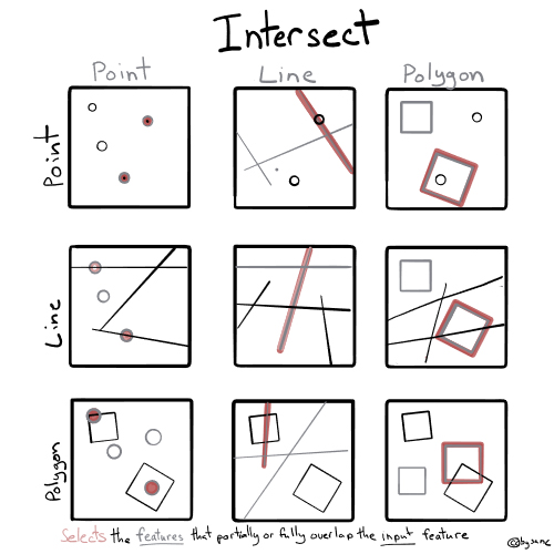
Intersecting Points with Polygons

Spatial data processing tools can understand the shared location of points and polygons to associate data from one dataset with another.

Objective: Associate a county name and identifier with each convenience store.

# Join county to store_geo
store_co_geo <- st_join(store_geo, us_co_filtered, join=st_intersects)

This operation may take some time depending on the machine you are working on. Just be patient.

Notice that store_co_geo has all of the observations from store_geo and has the corresponding variables from us_co attached to it. Now we have county information associated with the store location. We can join the convenience store data to census data or other data at the county level via the 5-digit FIPS. We can also aggregate convenience store information up to the county level using group_by() %>% summarize().

You Do It

Aggregate convenience store information up to the county level using group_by() %>% summarize() and plot the number of stores per county using mapview.

# Aggregate store count by county
store_count_by_county <- store_co_geo %>%
  group_by(geoid) %>%
  summarize(store_count = n(), .groups = 'drop')  # Drop groups to prevent regrouping

# Join aggregated data back with county geometries for mapping
county_store_map <- st_join(us_co_filtered,store_count_by_county,join=st_intersects)

# Visualize the result with mapview (showing number of stores per county)
mapview(county_store_map, zcol = "store_count")

Accessing U.S. Census data

The US Census contains a wealth of data that can be used in analysis. We will access median household income from the American Community Survey, an annual survey conducted to supplement the decennial census, using the R package called tidycensus that conveniently wraps the Census API (https://walker-data.com/tidycensus/). The Census stores many datasets, so we need to identify the one we want to use to represent median household income. Tidycensus provides a utility to find the table we want:

# Load variable metadata for the 2022 ACS 5-year estimates (used to look up variable codes and labels)
census_22 <- load_variables(2022, "acs5", cache = TRUE)

Use the filter feature in the R Studio viewer or export the data as a csv that you can open in Excel and search the descriptions. As you can see, there are many other demographic tables available in the Census data. In this case, the median household income code is B19013_001 (the table is B19013 and the variable we want is 001). We can access the data using the function get_acs().

# Download median household income data from the 2022 ACS 5-year estimates at the county level
census_hhi <- get_acs(
  geography = "county",                      # Get data for all U.S. counties
  survey = "acs5",                           # Use 5-year ACS data (more reliable for small areas)
  variables = c(medincome = "B19013_001"),   # B19013_001 = median household income
  state = NULL,                              # NULL = include all states (not just one)
  year = 2022                                # Use the most recent available year
)

# Clean column names and keep only GEOID and the income estimate, renamed as 'hhi'
hhi <- census_hhi %>%
  clean_names() %>%
  select(geoid, hhi = estimate)

This call to the API downloads county names and identifiers along with the variable estimate and margin of error.

Joining with Convenience Store County

We can join median household income to the stores by the common variable, geoid.

# Join median household income (hhi) to the store-level dataset using county GEOID
store_hhi <- store_co_geo %>%
  st_set_geometry(NULL) %>%        # Remove geometry to work with as a regular data frame
  inner_join(hhi, by = "geoid")    # Join on county identifier (GEOID)

We have added median household income to our store-level data. Export this data and visualize in Tableau.

Aggregating by Geography

Now we have the information to count the number of store in each county. We can use the group_by() and summarize() combination to calculate aggregate measures by county. Moreover, we don’t need the spatial information anymore since everything will be at the county level. We use st_set_geometry(NULL) to convert an sf object back to a data frame (without spatial information), then add the number of stores in a county.

# Count the number of stores per county by joining spatial store data with county identifiers
county_stores <- store_co_geo %>%
  st_set_geometry(NULL) %>%            # Drop geometry to simplify data manipulation
  group_by(geoid, county = name, state = stusps) %>%  # Group by county GEOID, name, and state abbreviation
  summarize(total_stores = n()) %>%    # Count the number of stores in each county
  ungroup()                            # Remove grouping to avoid unexpected behavior in downstream steps

The result, county_stores, contains the number of convenience stores in each county.

Creating a Panel

We may want to join our data to other data that varies over time. Suppose we are interested in how total sales at a store correlates with high temperatures. Weather data varies over time and space; however, store locations are fixed and do not change over time. We can use our existing data stores_co_geo, which has county information associated with each store, and join it to shopper_info, which contains the transaction level information. We need to aggregate the transaction level data up to sales per store-day.

# Read in the transaction level data
shopper_info <- read_csv("https://csu-arec-330.github.io/materials/unit_03/inputs/shopper_info.csv.gz")

# Read in the weather data
weather_raw <- read_csv("https://csu-arec-330.github.io/materials/unit_03/inputs/gridmet_county_daily_2023-2023.csv.gz")

shopper_info contains store_id, which we can use to join to store_co_geo, and date_time.

First, extract the date component as we are not concerned with the time of day. Then, we group by measure_date and store_id and sum sales (unit_price*unit_quantity)

# Aggregate daily sales by store from transaction-level data
store_sales <- shopper_info %>%
  mutate(measure_date = as_date(date_time)) %>%              # Extract date component from timestamp
  group_by(store_id, measure_date) %>%                       # Group by store and date
  summarize(
    sales = sum(unit_price * unit_quantity, na.rm = TRUE)   # Compute total sales (price × quantity)
  ) %>%
  ungroup()                                                  # Remove grouping to clean up the result

store_sales contains the total sales by date for each store in the dataset. We can now join store_sales with county information associated with each store.

# Add county GEOID to the store-level sales data (so we can link to county-level data like weather)
store_sales_co <- st_set_geometry(store_co_geo, NULL) %>%
  select(store_id, geoid) %>%                      # Keep only store_id (for joining) and geoid (for county-level linkage)
  inner_join(store_sales, ., by = "store_id")      # Join to sales data using store_id; keep only stores with known county info

We have county-day measurements of weather. However, the data is in long format (as opposed to wide). The unit of observation of weather_raw is county-day-weather_measurement, but we need it to be county-day with different measurements as columns. We can reshape this data from long to wide using the function pivot_wider().

The next step is to join the weather data with store_sales_co. However, the columns we need to join on have different names. We can rename them or tell R how to map the names.

Important Points before Joining Dataframes

1. The order of the variable name matters: The variable name on the left should be from the dataframe listed first.
2. The weather data is for the continental US so store locations outside of that will be dropped because of the inner_join().
   

# Reshape weather data from long to wide format (each variable becomes a column)
weather_wide <- weather_raw %>%
  pivot_wider(
    id_cols = c(county, date),              # Keep county and date as identifiers
    names_from = variable,                  # Each unique variable becomes a new column
    values_from = value                     # Fill those columns with the corresponding values
  )

# Join daily store sales to weather data using date and county identifiers
store_sales_weather <- store_sales_co %>%
  inner_join(weather_wide, by = c("measure_date" = "date", "geoid" = "county"))  # Match on date and county FIPS

Review the code associated with this week’s lab for more on how to combine shopper sales data with the weather data.

Summary

This lab demonstrates how to join spatial point data (convenience store locations) with spatial polygon data (county boundaries). Standard political boundaries like counties can be used as a common identifier to join US Census data. The lab also covered joining data that varies over space and time.

Lab Script for Week 13: Introduction to Panel Data Analysis and Spatial Data in R

# This is the R script for Week 13 Lab. 
# This script will demonstrate how to work with spatial data and conduct some basic operations (e.g., intersection)

# load packages
library(pacman)
p_load(tidyverse,janitor,sf,tigris,mapview,tidycensus,dplyr)

# ==== Read in Spatial Data ==== #

# Read in convenience store location dataset
store_raw <- read_csv("https://csu-arec-330.github.io/materials/unit_03/inputs/store_info.csv.gz")

# Convert data frame to a points simple feature object
store_geo <- store_raw %>%
  
  # First, we subset the variables `store_id` and the coordinates.
  select(store_id, latitude, longitude) %>% 
  
  # Tells R that these are essentially $x$ and $y$ coordinates in a certain projection (represented by the code 4326). See <https://epsg.io/> for more information.
  st_as_sf(coords=c("longitude","latitude"), crs = st_crs(4326))  

# Configure mapview to render points directly in the RStudio Viewer (not using flatgeobuf)
mapviewOptions(fgb = FALSE)

# Display the store locations as an interactive map
mapview(store_geo)

# Fetch data for county polygons using the 'tigris' package
us_co <- tigris::counties(cb=T,class="sf") %>%
  janitor::clean_names() %>%
  mutate(aland=aland/2.59e+6) %>%
  st_transform(4326)

mapview(us_co)

# Look at the distinct state list by statefp code
unique_statefp <- us_co %>%
  st_set_geometry(NULL) %>%  # Remove geometry column
  select(stusps, statefp) %>%  # Select the columns of interest
  distinct() %>%  # Remove duplicates, keeping only unique rows
  arrange(stusps)  # Arrange alphabetically by stusps

# Filter out counties from American Samoa (60), Guam (66), Saipan Municipality (69), Puerto Rico (72), Virgin Islands (78), Alaska (02), and Hawaii (15)
us_co_filtered <- us_co %>%
  filter(!statefp %in% c("60", "66", "72", "02", "15", "69", "78"))

# Use mapview to plot the county layer, excluding the specified states
mapview(us_co_filtered)

# Join county to store_geo
store_co_geo <- st_join(store_geo, us_co_filtered, join=st_intersects)

# Aggregate store count by county
store_count_by_county <- store_co_geo %>%
  group_by(geoid) %>%
  summarize(
    store_count = n(), 
    .groups = 'drop')  # Drop groups to prevent regrouping

# Join aggregated data back with county geometries for mapping
county_store_map <- st_join(us_co_filtered, store_count_by_county, join=st_intersects)

# Visualize the result with mapview (showing number of stores per county)
mapview(county_store_map, zcol = "store_count")

# ==== Spatial Joins - Census ==== #

# Load variable metadata for the 2022 ACS 5-year estimates (used to look up variable codes and labels)
census_22 <- load_variables(2022, "acs5", cache = TRUE)

# Download median household income data from the 2022 ACS 5-year estimates at the county level
census_hhi <- get_acs(
  geography = "county",                      # Get data for all U.S. counties
  survey = "acs5",                           # Use 5-year ACS data (more reliable for small areas)
  variables = c(medincome = "B19013_001"),   # B19013_001 = median household income
  state = NULL,                              # NULL = include all states (not just one)
  year = 2022                                # Use the most recent available year
)

# Clean column names and keep only GEOID and the income estimate, renamed as 'hhi'
hhi <- census_hhi %>%
  clean_names() %>%
  select(geoid, hhi = estimate)

# Join median household income (hhi) to the store-level dataset using county GEOID
store_hhi <- store_co_geo %>%
  st_set_geometry(NULL) %>%        # Remove geometry to work with as a regular data frame
  inner_join(hhi, by = "geoid")    # Join on county identifier (GEOID)

# Count the number of stores per county by joining spatial store data with county identifiers
county_stores <- store_co_geo %>%
  st_set_geometry(NULL) %>%            # Drop geometry to simplify data manipulation
  group_by(geoid, county = name, state = stusps) %>%  # Group by county GEOID, name, and state abbreviation
  summarize(
    total_stores = n()
    ) %>%    # Count the number of stores in each county
  ungroup()                            # Remove grouping to avoid unexpected behavior in downstream steps

# ==== Spatial Joins - Weather ==== #

# Read in the transaction level data
shopper_info <- read_csv("https://csu-arec-330.github.io/materials/unit_03/inputs/shopper_info.csv.gz")

# Read in the weather data
weather_raw <- read_csv("https://csu-arec-330.github.io/materials/unit_03/inputs/gridmet_county_daily_2023-2023.csv.gz")

# ==== Store-related questions ==== #

# Aggregate daily sales by store from transaction-level data
store_sales <- shopper_info %>%
  mutate(gtin = ifelse(is.na(gtin), 0, gtin)) %>%
  mutate(measure_date = as_date(date_time)) %>%              # Extract date component from timestamp
  group_by(store_id, measure_date) %>%                       # Group by store and date
  summarize(
    sales = sum(unit_price * unit_quantity, na.rm = TRUE)   # Compute total sales (price × quantity)
  ) %>%
  ungroup()                                                  # Remove grouping to clean up the result

# Add county GEOID to the store-level sales data (so we can link to county-level data like weather)
store_sales_co <- st_set_geometry(store_co_geo, NULL) %>%
  select(store_id, geoid) %>%                      # Keep only store_id (for joining) and geoid (for county-level linkage)
  inner_join(store_sales, ., by = "store_id")      # Join to sales data using store_id; keep only stores with known county info

# Reshape weather data from long to wide format (each variable becomes a column)
weather_wide <- weather_raw %>%
  pivot_wider(
    id_cols = c(county, date),              # Keep county and date as identifiers
    names_from = variable,                  # Each unique variable becomes a new column
    values_from = value                     # Fill those columns with the corresponding values
  )

# Join daily store sales to weather data using date and county identifiers
store_sales_weather <- store_sales_co %>%
  inner_join(weather_wide, by = c("measure_date" = "date", "geoid" = "county"))  # Match on date and county FIPS

# Results in a data frame of daily sales at the store level with daily precipitation levels, humidity levels, and air temperature.

# ==== Shopper-related questions ==== #

# First need to assign location information to each shopper
shopper_home_co <- shopper_info %>%
  left_join(store_co_geo %>% select(store_id, geoid), by = "store_id") %>%
  filter(!is.na(geoid)) %>%
  group_by(shopper_id, geoid) %>%
  summarize(
    visits = n(), 
    .groups = "drop") %>%
  group_by(shopper_id) %>%
  filter(visits == max(visits)) %>% # Assign the shopper to the county of the store they most frequently visit
  ungroup() %>%
  distinct(shopper_id, .keep_all = TRUE) %>%
  select(shopper_id, home_co = geoid)

shopper_sales <- shopper_info %>%
  mutate(
    gtin = ifelse(is.na(gtin), 0, gtin),     # Replace NA with 0, ensure numeric
    measure_date = as_date(date_time)                    # Extract date from timestamp
  ) %>%
  group_by(shopper_id, measure_date) %>%
  summarize(
    total_spent = sum(unit_price * unit_quantity, na.rm = TRUE),
    visit_count = n(),
    .groups = "drop"
  ) %>%
  left_join(shopper_home_co, by = "shopper_id")  # Add home county

# Reshape weather data from long to wide format (each variable becomes a column)
weather_wide <- weather_raw %>%
  pivot_wider(
    id_cols = c(county, date),              # Keep county and date as identifiers
    names_from = variable,                  # Each unique variable becomes a new column
    values_from = value                     # Fill those columns with the corresponding values
  )

# Join daily store sales to weather data using date and county identifiers
shopper_sales_weather <- shopper_sales %>%
  inner_join(weather_wide, by = c("measure_date" = "date", "home_co" = "county"))  # Match on date and county FIPS

# Results in a data frame of daily expenditures at the shopper level with daily precipitation levels, humidity levels, and air temperature.

Footnotes

1. Spatial data can also have temporal dimensions, and the concepts we cover here extend to those data too.