Week 14:
Regression Analysis and Hypothesis Testing

Agenda

Linear Regression

Hypothesis testing

Recap

Last week (week 13) we covered:

• Reading in spatial data
• Understanding and implementing spatial joins
• Building panel datasets for regression analysis

Why this is important: Researchers might want to control for geographic variation in the outcome variable.

This week: Apply regression analysis to panel data.

Linear Regression

The objective:
We want to understand the
relationship between two variables.

The simple solution:
Assume the relationship is linear
and estimate the “average” trend.

Linear regression: The intuition

Imagine you’re trying to figure out a relationship between two things:

• What is the relationship (correlation, association) between \(x\) (explanatory variable) and \(y\) (outcome)?

For instance, what is the association between the number of hours you study (\(x\)) and your test score (\(y\))?

• Hypothesis: The more you study, the better your score \(\rightarrow\) positively related.

Linear regression helps us quantify this relationship.

• For each additional hour studied, by how many points will my test score increase?

Equation of a line

Quick review: The equation of a line plotting the relationship between \(y\) and \(x\) is, \[y=mx+b \]

Which variable represents the slope?

Which variable represents the intercept?

ggplot(df, aes(x, y)) + 
  geom_line() +
  scale_y_continuous(
    breaks = seq.int(0, 24, 2),
    limits = c(0, 24),
    expand = c(0, 0)
  ) +
  scale_x_continuous(
    breaks = seq.int(0, 10, 2),
    expand = c(0, 0)
  ) +
  theme_bw(base_size = 15) +
  theme(
    axis.line = element_line(color = "black"),   # Draw axis lines
    panel.border = element_blank()               # Remove default plot border
  )

General Expression of a Regression Equation

The equation of a regression line is very similar to the equation of a line:

\[y= \beta_0 + \beta_1 x + \varepsilon ;~~ \varepsilon \sim N(0,1)\]

• \(\beta_0\) is our intercept
• \(\beta_1\) is our slope

Studying and Test Scores

Our data: We observe hours studied and test scores

• Plotted on the right using ggpairs() (Always plot your data!)

Scatter plot

Our data: We observe hours studied and test scores

What is the apparent relationship?

• Slope?
• Intercept?

\[y= \beta_0 + \beta_1~x + \varepsilon \]

What is Ordinary Least Squares (OLS)?

• OLS is a method for estimating the relationship between one or more independent variables and a dependent variable.

• It finds the best-fitting line by minimizing the sum of squared differences between the observed values and the predicted values.

• The goal is to find coefficients (slopes and intercept) that make the model’s predictions as close as possible to the actual data.

• Assumes that errors are normally distributed with constant variance and that there is a linear relationship between predictors and outcome.

How does OLS estimate regression coefficients? Shiny app

Estimate Regression

m_out

	(1)
+ p < 0.1, * p < 0.05, ** p < 0.01, *** p < 0.001
Intercept	40.389***
	(2.895)
Hours Studied	0.783***
	(0.090)
Num.Obs.	133
R2	0.364

In lab, we will learn about lm() which is the function that estimates a linear regression that generates this regression output.

True model vs estimates

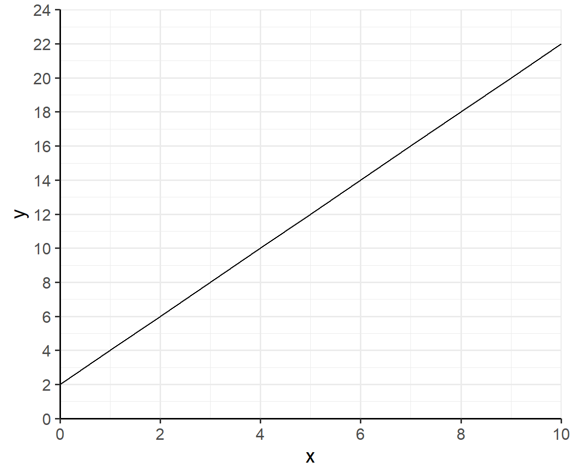
We use the regression output to construct our linear regression model:

\[scores=40 + 0.8 * hours + \varepsilon ;~~ \varepsilon \sim N(0,1)\]

	(1)
+ p < 0.1, * p < 0.05, ** p < 0.01, *** p < 0.001
Intercept	40.389***
	(2.895)
Hours Studied	0.783***
	(0.090)
Num.Obs.	133
R2	0.364

How well does our model fit?

R² is a statistic used to measures the proportion of variance in the dependent variable that is predictable from the independent variables

\[ R^2 = \frac{Explained ~~ Variation}{Total ~~ Variation} \]

The value of R² ranges from 0 to 1:

• 0 means that the model explains none of the variability of the response data around its mean.

• 1 means that the model explains all the variability of the response data around its mean.

Intuitive Explanation Imagine you are a teacher trying to understand the performance of your students on a test. You suspect that several factors like hours of study, attendance, and participation in class could influence test scores.

Here’s how R2 fits into this scenario:

Total Variation: First, look at the variation in test scores among all students. Some score high, some low, and many in the middle. This spread of scores is the “total variation” in your dataset.

Explained Variation: Now, suppose you create a statistical model that attempts to predict these scores based on the factors you think might affect them (study hours, attendance, etc.). After applying your model, some of this total variation in test scores will be “explained” by the factors in your model. For example, perhaps students who study more and attend regularly score higher.

Unexplained Variation: There’s almost always some part of the variation that your model can’t explain. Maybe some students do well on tests because they’re just good test-takers or they have a strong background in the subject that wasn’t measured.

Putting the coefficients on trial

Did we observe our estimate by chance or can we trust it?

The Hypotheses:

\(H_0\) (Null Hypothesis): posits that the regression coefficient is equal to zero.

• There is no effect of the independent variable (e.g., hours studied) on the dependent variable (e.g., test scores).

\(H_A\) (Alternative Hypothesis): posits that the coefficient is not zero.

• There there is an effect, and this effect is different from zero. The amount of studying does influence test scores.

Testing the hypothesis

We use a t-test to determine whether the regression coefficients are significantly different from zero.

The t-statistic is a ratio. The numerator is the difference between the estimated coefficient and zero (or other null hypothesis). The denominator is the standard error of the coefficient.

\[ t = \frac{\beta - 0}{se} = \frac{0.783 - 0}{0.09} = 8.7 \]

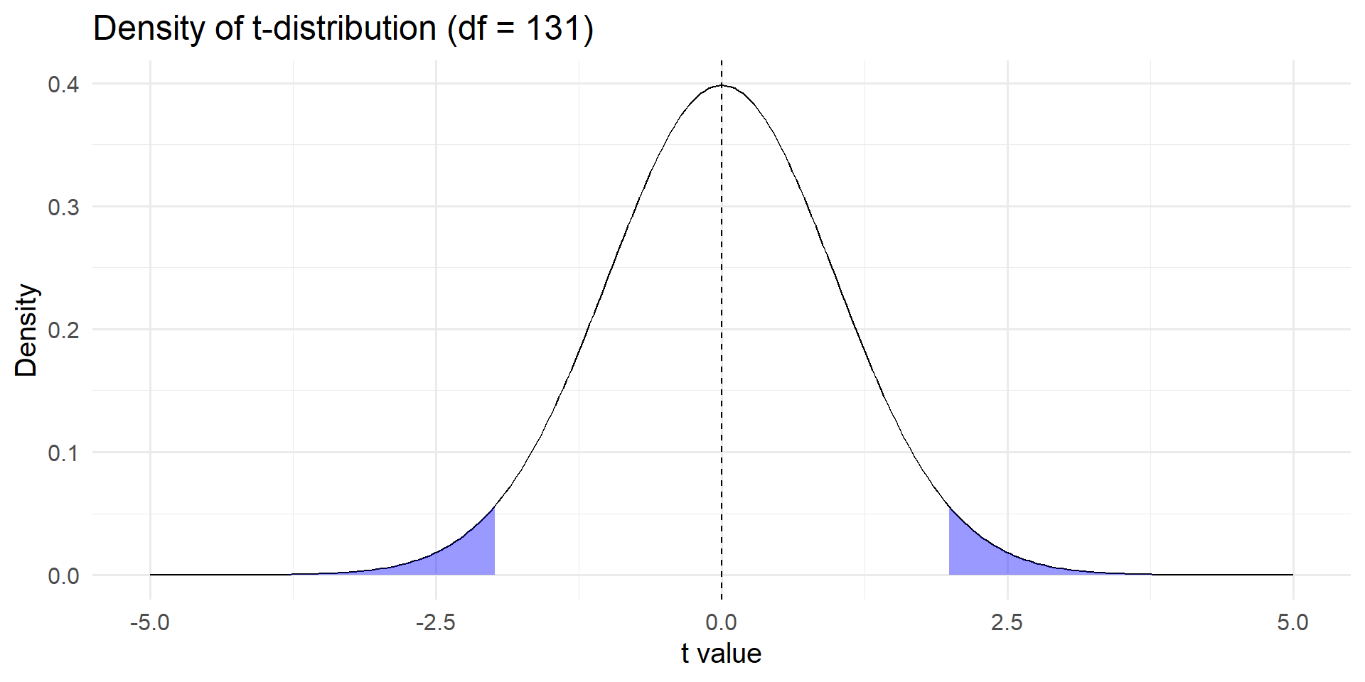
Student’s t-distribution

The shaded area is the probability that we observe the value by chance (p-value)

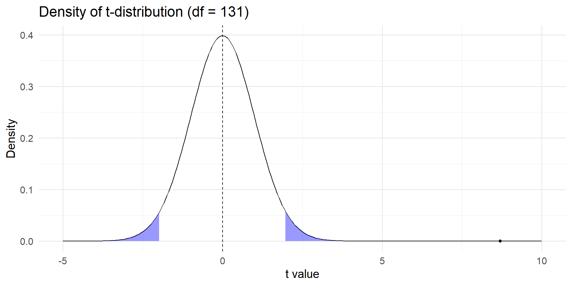
Student’s t-distribution

Locating our t-statistic on the density of the t-distribution quantifies the probability that we observe our result by chance (p-val = 1.199041e-14)

95% Confidence Interval

Reverse engineer the p-value of 0.05 to find the test statistic (1.96)

\[ 1.96 = \frac{\beta - 0}{se} \]

Then rearrange the t-statistics calculation

\[ upper = \beta + 1.96*se ; ~~~ lower = \beta - 1.96*se\]

Inference - back to the trial

The p-val = 0.00000000000001199041 suggests the probability of observing the relationship between studying and test score by chance is small.

Formally, we reject the null hypothesis H0 (no relationship) at an alpha=.05

Our test does not prove that H1 is correct, but it provides strong evidence.

Interpreting regression coefficients

	(1)
+ p < 0.1, * p < 0.05, ** p < 0.01, *** p < 0.001
Intercept	40.389***
	(2.895)
Hours Studied	0.783***
	(0.090)
Num.Obs.	133
R2	0.364

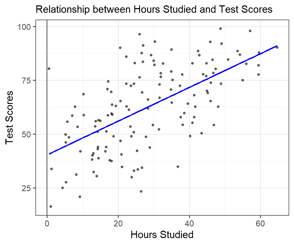
A student that does not study is expected to get a score of 40.389.

A student’s score should improve by 0.78 points per hour of additional studying.

How many hours should a student study to get 80 points or better?

Predicting new values

We can use the coefficient estimates to calculate expected scores from new students based on study time

\[scores=40 + 0.78 * hours \]

Multivariate regression

You can add additional independent variables (a.k.a. regressors).

\[ y=\alpha + \beta_1 X_1 + \beta_2 X_2 + ... +\varepsilon \]

The \(\beta\)’s are conditional on the other covariates.

Inference is similar.

Summary

Regression is a tool to estimate relationships between variables (measurements)

When assumptions are met, the regression provides the best estimates of the relationship

Hypothesis testing helps us understand the quality of our estimates

Project 3

Option 1:
What is the relationship between
median income and total store count
at the county level?

Plot Your Data

p_load(GGally)

# Basic scatter plot with ggplot
county_hhi %>%
  st_set_geometry(NULL) %>%
  mutate(store_count = replace_na(store_count, 0)) %>%
  select(hhi, store_count) %>%
  ggpairs()

Zoom in on Scatter Plot

Estimate Regression

m_out

	(1)
+ p < 0.1, * p < 0.05, ** p < 0.01, *** p < 0.001
Intercept	-4.38605***
	(1.00645)
Median Inc	0.00019***
	(0.00002)
Num.Obs.	3108
R2	0.046

:::

Linear Regression Model

\[StoreCount= -4.38605 + 0.00019 * MedianIncome + \varepsilon ;~~ \varepsilon \sim N(0,1)\]

	(1)
+ p < 0.1, * p < 0.05, ** p < 0.01, *** p < 0.001
Intercept	-4.38605***
	(1.00645)
Median Inc	0.00019***
	(0.00002)
Num.Obs.	3108
R2	0.046

Interpreting the Results

1. The \(R^2\) is very low at 0.046, meaning that median income does not explain much of the variation in store count. In general, this is not a well-fitted model.

2. The intercept (\(\beta_0\)) is −4.38605, meaning that when median income=0, the model predicts a negative store count. Since an income of 0 isn’t meaningful, the intercept mainly acts as a mathematical anchor. (We usually don’t over-interpret it here.)

3. The slope (\(\beta_1\)) is 0.00019, meaning that for every 1 unit increase in median income, store count increases by 0.00019.

• One way to make this more interpretable is to imagine that median income increases by $10,000. Then, we would expect store count to increase by 1.9 (because 10,000 \(\times\) 0.00019 = 1.9), which is almost 2 stores. At the county level, this could make sense.

Action Items

If we take these results to be true, we might suggest to a policymaker that higher median income areas are slightly more likely to attract more stores.

However, given the low \(R^2\), other factors likely play a much larger role in determining store count.

Further steps could include:

• Using a multivariate model to better capture the drivers of store count variation by adding more predictors (e.g., population density, rural or urban status, infrastructure).